```{r}
#| include: false
suppressPackageStartupMessages(library(tidyverse))
suppressPackageStartupMessages(library(knitr))
source(normalizePath(file.path(dirname(knitr::current_input(dir = TRUE)), "..", "R", "chapter_table_helpers.R"), mustWork = TRUE))
# AHP criteria comparisons: Cost, Effectiveness, Feasibility.
criteria_names <- c("Cost", "Effectiveness", "Feasibility")
ahp_matrix <- matrix(
c(
1, 1/3, 1/1.5,
3, 1, 2,
1.5, 1/2, 1
),
nrow = 3,
byrow = TRUE,
dimnames = list(criteria_names, criteria_names)
)
eig <- eigen(ahp_matrix)
principal <- Re(eig$vectors[, 1])
criteria_weights <- principal / sum(principal)
names(criteria_weights) <- criteria_names
lambda_max <- Re(eig$values[1])
consistency_index <- (lambda_max - length(criteria_names)) / (length(criteria_names) - 1)
random_index <- 0.58
consistency_ratio <- max(consistency_index, 0) / random_index
criteria_table <- tibble(
Criterion = criteria_names,
Weight = formatC(criteria_weights, format = "f", digits = 3),
`Relative emphasis` = c("Cost matters, but is not dominant", "Primary criterion", "Secondary practical criterion")
)
programme_scores <- tibble(
Programme = c("A", "B", "C"),
Cost = c(0.50, 0.30, 0.20),
Effectiveness = c(0.25, 0.50, 0.25),
Feasibility = c(0.40, 0.30, 0.30)
) %>%
mutate(
`Weighted cost` = Cost * criteria_weights["Cost"],
`Weighted effectiveness` = Effectiveness * criteria_weights["Effectiveness"],
`Weighted feasibility` = Feasibility * criteria_weights["Feasibility"],
`Total score` = `Weighted cost` + `Weighted effectiveness` + `Weighted feasibility`
) %>%
arrange(desc(`Total score`)) %>%
mutate(Rank = row_number())
ahp_display <- programme_scores %>%
transmute(
Rank,
Programme,
`Weighted cost` = formatC(`Weighted cost`, format = "f", digits = 3),
`Weighted effectiveness` = formatC(`Weighted effectiveness`, format = "f", digits = 3),
`Weighted feasibility` = formatC(`Weighted feasibility`, format = "f", digits = 3),
`Total score` = formatC(`Total score`, format = "f", digits = 3)
)
decision_matrix <- tibble(
Project = c("P1", "P2", "P3", "P4"),
Impact = c(7, 8, 6, 9),
Cost = c(50, 70, 40, 80),
Support = c(6, 7, 8, 7)
)
weights_topsis <- c(Impact = 1/3, Cost_benefit = 1/3, Support = 1/3)
topsis_work <- decision_matrix %>%
mutate(Cost_benefit = max(Cost) - Cost + min(Cost))
criteria_cols <- c("Impact", "Cost_benefit", "Support")
normalised <- topsis_work %>%
mutate(across(all_of(criteria_cols), ~ .x / sqrt(sum(.x^2)), .names = "norm_{.col}"))
weighted <- normalised %>%
mutate(
w_Impact = norm_Impact * weights_topsis["Impact"],
w_Cost = norm_Cost_benefit * weights_topsis["Cost_benefit"],
w_Support = norm_Support * weights_topsis["Support"]
)
ideal <- c(max(weighted$w_Impact), max(weighted$w_Cost), max(weighted$w_Support))
negative_ideal <- c(min(weighted$w_Impact), min(weighted$w_Cost), min(weighted$w_Support))
topsis_results <- weighted %>%
rowwise() %>%
mutate(
`Distance to ideal` = sqrt((w_Impact - ideal[1])^2 + (w_Cost - ideal[2])^2 + (w_Support - ideal[3])^2),
`Distance to negative ideal` = sqrt((w_Impact - negative_ideal[1])^2 + (w_Cost - negative_ideal[2])^2 + (w_Support - negative_ideal[3])^2),
`Closeness coefficient` = `Distance to negative ideal` / (`Distance to ideal` + `Distance to negative ideal`)
) %>%
ungroup() %>%
arrange(desc(`Closeness coefficient`)) %>%
mutate(Rank = row_number())
topsis_display <- topsis_results %>%
transmute(
Rank,
Project,
Impact,
Cost,
Support,
`Closeness coefficient` = formatC(`Closeness coefficient`, format = "f", digits = 3)
)
vikor_scaled <- topsis_work %>%
transmute(
Project,
Impact = weights_topsis["Impact"] *
(max(Impact) - Impact) / (max(Impact) - min(Impact)),
Cost_benefit = weights_topsis["Cost_benefit"] *
(max(Cost_benefit) - Cost_benefit) / (max(Cost_benefit) - min(Cost_benefit)),
Support = weights_topsis["Support"] *
(max(Support) - Support) / (max(Support) - min(Support))
)
vikor_raw <- vikor_scaled %>%
mutate(
S = Impact + Cost_benefit + Support,
R = pmax(Impact, Cost_benefit, Support)
)
vikor_v <- 0.5
vikor_results <- vikor_raw %>%
mutate(
Q = vikor_v * (S - min(S)) / (max(S) - min(S)) +
(1 - vikor_v) * (R - min(R)) / (max(R) - min(R))
) %>%
arrange(Q) %>%
mutate(Rank = row_number())
vikor_display <- vikor_results %>%
transmute(
Rank,
Project,
`Utility loss (S)` = formatC(S, format = "f", digits = 3),
`Regret loss (R)` = formatC(R, format = "f", digits = 3),
`VIKOR index (Q)` = formatC(Q, format = "f", digits = 3)
)
sensitivity_results <- map_dfr(seq(0.30, 0.80, by = 0.05), function(eff_weight) {
remaining <- 1 - eff_weight
cost_weight <- remaining * (criteria_weights["Cost"] / (criteria_weights["Cost"] + criteria_weights["Feasibility"]))
feas_weight <- remaining * (criteria_weights["Feasibility"] / (criteria_weights["Cost"] + criteria_weights["Feasibility"]))
scores <- programme_scores %>%
transmute(
Programme,
Score = Cost * cost_weight + Effectiveness * eff_weight + Feasibility * feas_weight
) %>%
arrange(desc(Score))
tibble(
`Effectiveness weight` = eff_weight,
`Top programme` = scores$Programme[1],
`Top score` = scores$Score[1],
Ranking = paste(scores$Programme, collapse = " > ")
)
})
sensitivity_display <- sensitivity_results %>%
transmute(
`Effectiveness weight` = formatC(`Effectiveness weight`, format = "f", digits = 2),
`Top programme`,
Ranking
)
sensitivity_plot <- ggplot(sensitivity_results, aes(x = `Effectiveness weight`, y = `Top score`, colour = `Top programme`)) +
geom_line(linewidth = 0.8) +
geom_point(size = 2.1) +
scale_x_continuous(breaks = seq(0.30, 0.80, by = 0.10)) +
labs(
x = "Weight assigned to effectiveness",
y = "Score of top-ranked programme",
title = "AHP ranking sensitivity to the effectiveness weight"
) +
theme_classic(base_size = 12) +
theme(legend.position = "top", plot.title = element_text(size = 13))
```
# Chapter 14: Multi-Criteria Decision Making (MCDM) for Small Sets of Alternatives
### Learning Objectives
By the end of this chapter, you will be able to distinguish decision analysis from statistical inference, structure a small multi-criteria decision problem, compute transparent weighted rankings with AHP and TOPSIS, check consistency and sensitivity, and report rankings without implying more precision than stakeholder judgements support.
### When MCDM Methods Are Appropriate
Multi-criteria decision-making methods are useful when a small set of alternatives must be ranked or selected using several criteria. Their value lies in transparency: the criteria, weights, normalisation choices, and aggregation rule are all visible, so stakeholders can see how a ranking was produced and whether it holds under plausible assumptions. They produce ranked or weighted scores rather than p-values or population-parameter estimates.
MCDM belongs in a small-sample methods text because many constrained research settings end with a decision rather than a population estimate. A school may need to choose one of three reading interventions, a clinic may need to prioritise one of four service improvements, or a community project may need to allocate a small grant among a few feasible options. When the alternatives are fixed and the evidence is too limited for strong inference, a structured decision model is more honest than pretending that a p-value can select the best option.
MCDM is appropriate when alternatives are few, criteria are heterogeneous, stakeholder preferences matter, and the goal is selection or resource allocation [@saaty1980; @hwang1981]. When the question is whether a treatment caused an effect, only a controlled experiment can answer it.
### Analytic Hierarchy Process
The Analytic Hierarchy Process (AHP) uses pairwise comparisons to derive priority weights [@saaty1980]. Decision-makers compare criteria two at a time, and the resulting matrix is converted into weights. AHP also includes a consistency check. A low consistency ratio suggests that the pairwise judgements are coherent enough to use. A high value means the comparisons should be revisited.
Before constructing the matrix, document the elicitation protocol: who supplied the comparisons, what scale was used, whether judgements were individual or consensus-based, and how disagreements were resolved. A simple stakeholder template should ask each rater to compare every pair of criteria, give a short reason for each judgement, and flag any comparison they feel uncertain about. The final matrix should be auditable rather than treated as a hidden expert input.
Table 14.1 gives the criteria weights for a training-programme selection example. Effectiveness receives the largest weight, while cost and feasibility still contribute to the decision.
The AHP calculation below uses the principal eigenvector of the pairwise-comparison matrix. The consistency ratio is computed as `(lambda_max - k) / ((k - 1) * RI)`, where `k` is the number of criteria and `RI` is Saaty's random-index value for a matrix of that size.
:::: {.content-visible when-format="html"}
```{webr-r}
#| label: ch14-ahp-code-template
#| context: interactive
criteria_names <- c("Cost", "Effectiveness", "Feasibility")
ahp_matrix <- matrix(
c(
1, 1/3, 1/1.5,
3, 1, 2,
1.5, 1/2, 1
),
nrow = 3,
byrow = TRUE,
dimnames = list(criteria_names, criteria_names)
)
eig <- eigen(ahp_matrix)
weights <- Re(eig$vectors[, 1])
weights <- weights / sum(weights)
lambda_max <- Re(eig$values[1])
consistency_index <- (lambda_max - length(criteria_names)) / (length(criteria_names) - 1)
consistency_ratio <- consistency_index / 0.58
round(weights, 3)
round(consistency_ratio, 3)
```
::::
:::: {.content-visible unless-format="html"}
```{r}
#| eval: false
#| label: ch14-ahp-code-template-pdf
criteria_names <- c("Cost", "Effectiveness", "Feasibility")
ahp_matrix <- matrix(
c(
1, 1/3, 1/1.5,
3, 1, 2,
1.5, 1/2, 1
),
nrow = 3,
byrow = TRUE,
dimnames = list(criteria_names, criteria_names)
)
eig <- eigen(ahp_matrix)
weights <- Re(eig$vectors[, 1])
weights <- weights / sum(weights)
lambda_max <- Re(eig$values[1])
consistency_index <- (lambda_max - length(criteria_names)) / (length(criteria_names) - 1)
consistency_ratio <- consistency_index / 0.58
```
::::
```{r}
#| label: ch14-criteria-table
#| echo: false
#| results: asis
smallsamplelab_apa_table(
"14.1",
"AHP criteria weights for the training-programme decision",
criteria_table,
note = sprintf(
"The consistency ratio is %.3f. A CR below 0.10 is commonly treated as acceptable for pairwise-comparison matrices (Saaty, 1980). For very small 3 x 3 matrices, some authors tolerate slightly higher values, but inconsistent judgements should still be revisited.",
consistency_ratio
),
align = c("l", "r", "l")
)
```
```{r}
#| label: ch14-ahp-table
#| echo: false
#| results: asis
smallsamplelab_apa_table(
"14.2",
"AHP weighted scores for three training programmes",
ahp_display,
note = "Programme B ranks highest because effectiveness has the largest weight and Programme B performs best on that criterion.",
align = c("r", "l", "r", "r", "r", "r")
)
```
Interpretation should be decision-focused rather than inferential. Programme B is the preferred option under the stated weights and scores. That does not mean Programme B is statistically superior. It means the explicit decision model ranks it highest.
### TOPSIS
TOPSIS ranks alternatives by closeness to an ideal solution and distance from a negative-ideal solution [@hwang1981]. The method first normalises the criteria, applies weights, identifies the best and worst value on each weighted criterion, and then computes a closeness coefficient. Higher coefficients indicate alternatives closer to the ideal profile.
Cost criteria require recoding because TOPSIS assumes larger values are better. In Table 14.3, project cost is transformed into a benefit score before normalisation.
The vector-normalisation step divides each criterion value by the Euclidean norm of its column:
$$
r_{ij} = \frac{x_{ij}}{\sqrt{\sum_i x_{ij}^2}}.
$$
The implementation below shows the full calculation, including the cost-to-benefit transformation and closeness coefficient.
:::: {.content-visible when-format="html"}
```{webr-r}
#| label: ch14-topsis-code-template
#| context: interactive
library(dplyr)
decision_matrix <- tibble(
Project = c("P1", "P2", "P3", "P4"),
Impact = c(7, 8, 6, 9),
Cost = c(50, 70, 40, 80),
Support = c(6, 7, 8, 7)
)
weights_topsis <- c(Impact = 1/3, Cost_benefit = 1/3, Support = 1/3)
topsis_work <- decision_matrix |>
mutate(Cost_benefit = max(Cost) - Cost + min(Cost))
normalised <- topsis_work |>
mutate(across(c(Impact, Cost_benefit, Support),
~ .x / sqrt(sum(.x^2)),
.names = "norm_{.col}"))
weighted <- normalised |>
mutate(
w_Impact = norm_Impact * weights_topsis["Impact"],
w_Cost = norm_Cost_benefit * weights_topsis["Cost_benefit"],
w_Support = norm_Support * weights_topsis["Support"]
)
ideal <- c(max(weighted$w_Impact), max(weighted$w_Cost), max(weighted$w_Support))
negative_ideal <- c(min(weighted$w_Impact), min(weighted$w_Cost), min(weighted$w_Support))
topsis_results <- weighted |>
rowwise() |>
mutate(
distance_ideal = sqrt(sum((c(w_Impact, w_Cost, w_Support) - ideal)^2)),
distance_negative = sqrt(sum((c(w_Impact, w_Cost, w_Support) - negative_ideal)^2)),
closeness = distance_negative / (distance_ideal + distance_negative)
) |>
ungroup() |>
arrange(desc(closeness))
topsis_results |>
select(Project, closeness)
```
::::
:::: {.content-visible unless-format="html"}
```{r}
#| eval: false
#| label: ch14-topsis-code-template-pdf
decision_matrix <- tibble(
Project = c("P1", "P2", "P3", "P4"),
Impact = c(7, 8, 6, 9),
Cost = c(50, 70, 40, 80),
Support = c(6, 7, 8, 7)
)
weights_topsis <- c(Impact = 1/3, Cost_benefit = 1/3, Support = 1/3)
topsis_work <- decision_matrix |>
mutate(Cost_benefit = max(Cost) - Cost + min(Cost))
normalised <- topsis_work |>
mutate(across(c(Impact, Cost_benefit, Support),
~ .x / sqrt(sum(.x^2)),
.names = "norm_{.col}"))
weighted <- normalised |>
mutate(
w_Impact = norm_Impact * weights_topsis["Impact"],
w_Cost = norm_Cost_benefit * weights_topsis["Cost_benefit"],
w_Support = norm_Support * weights_topsis["Support"]
)
ideal <- c(max(weighted$w_Impact), max(weighted$w_Cost), max(weighted$w_Support))
negative_ideal <- c(min(weighted$w_Impact), min(weighted$w_Cost), min(weighted$w_Support))
topsis_results <- weighted |>
rowwise() |>
mutate(
distance_ideal = sqrt(sum((c(w_Impact, w_Cost, w_Support) - ideal)^2)),
distance_negative = sqrt(sum((c(w_Impact, w_Cost, w_Support) - negative_ideal)^2)),
closeness = distance_negative / (distance_ideal + distance_negative)
) |>
ungroup() |>
arrange(desc(closeness))
```
::::
```{r}
#| label: ch14-topsis-table
#| echo: false
#| results: asis
smallsamplelab_apa_table(
"14.3",
"TOPSIS ranking for four community projects",
topsis_display,
note = "Cost was recoded as a benefit before vector normalisation, where each criterion value is divided by the Euclidean norm of its column. This places criteria on a comparable scale before weighting. The closeness coefficient ranges from 0 to 1.",
align = c("r", "l", "r", "r", "r", "r")
)
```
The TOPSIS ranking depends on the normalisation rule and the weights. If stakeholders disagree about cost or impact weights, the ranking should be recomputed under those alternatives rather than reported as a single unquestioned answer.
### VIKOR and Other MCDM Methods
VIKOR is another ideal-solution method, but it emphasises compromise between group utility and individual regret [@opricovic2004]. TOPSIS asks which alternative is geometrically closest to the ideal profile. VIKOR asks which alternative is a defensible compromise when no option is best on every criterion. Other methods, such as SMART, WASPAS, and MOORA, follow the same broad logic: structure the decision, normalise criteria, apply weights, aggregate scores, and test sensitivity.
The VIKOR calculation below uses the same four projects and equal criterion weights as the TOPSIS example. For each criterion, the best value receives zero loss and worse values receive larger normalised loss. The utility measure `S` summarises total weighted loss, the regret measure `R` records the largest single-criterion loss, and the index `Q` combines both using `v = 0.5` to balance group utility and individual regret. Lower `Q` values are preferred.
:::: {.content-visible when-format="html"}
```{webr-r}
#| label: ch14-vikor-code-template
#| context: interactive
library(dplyr)
decision_matrix <- tibble(
Project = c("P1", "P2", "P3", "P4"),
Impact = c(7, 8, 6, 9),
Cost = c(50, 70, 40, 80),
Support = c(6, 7, 8, 7)
)
weights_topsis <- c(Impact = 1/3, Cost_benefit = 1/3, Support = 1/3)
topsis_work <- decision_matrix |>
mutate(Cost_benefit = max(Cost) - Cost + min(Cost))
vikor_scaled <- topsis_work |>
transmute(
Project,
Impact = weights_topsis["Impact"] *
(max(Impact) - Impact) / (max(Impact) - min(Impact)),
Cost_benefit = weights_topsis["Cost_benefit"] *
(max(Cost_benefit) - Cost_benefit) / (max(Cost_benefit) - min(Cost_benefit)),
Support = weights_topsis["Support"] *
(max(Support) - Support) / (max(Support) - min(Support))
) |>
mutate(
S = Impact + Cost_benefit + Support,
R = pmax(Impact, Cost_benefit, Support),
Q = 0.5 * (S - min(S)) / (max(S) - min(S)) +
0.5 * (R - min(R)) / (max(R) - min(R))
) |>
arrange(Q)
vikor_scaled |>
select(Project, S, R, Q)
```
::::
:::: {.content-visible unless-format="html"}
```{r}
#| eval: false
#| label: ch14-vikor-code-template-pdf
vikor_scaled <- topsis_work |>
transmute(
Project,
Impact = weights_topsis["Impact"] *
(max(Impact) - Impact) / (max(Impact) - min(Impact)),
Cost_benefit = weights_topsis["Cost_benefit"] *
(max(Cost_benefit) - Cost_benefit) / (max(Cost_benefit) - min(Cost_benefit)),
Support = weights_topsis["Support"] *
(max(Support) - Support) / (max(Support) - min(Support))
) |>
mutate(
S = Impact + Cost_benefit + Support,
R = pmax(Impact, Cost_benefit, Support),
Q = 0.5 * (S - min(S)) / (max(S) - min(S)) +
0.5 * (R - min(R)) / (max(R) - min(R))
) |>
arrange(Q)
```
::::
```{r}
#| label: ch14-vikor-table
#| echo: false
#| results: asis
smallsamplelab_apa_table(
"14.4",
"VIKOR compromise ranking for the community project example",
vikor_display,
note = "Lower Q values are preferred. Compare this compromise ranking with the TOPSIS closeness ranking. Disagreement is a sensitivity finding, not an error.",
align = c("r", "l", "r", "r", "r")
)
```
The technical differences matter less than the reporting discipline. Always state the criteria and their substantive justification, the raw scores and direction of preference, the weights and how they were elicited, the normalisation and aggregation methods, and sensitivity analyses across plausible weight sets. Weights are value judgements, not statistical estimates, so they need transparent justification.
### Sensitivity Analysis
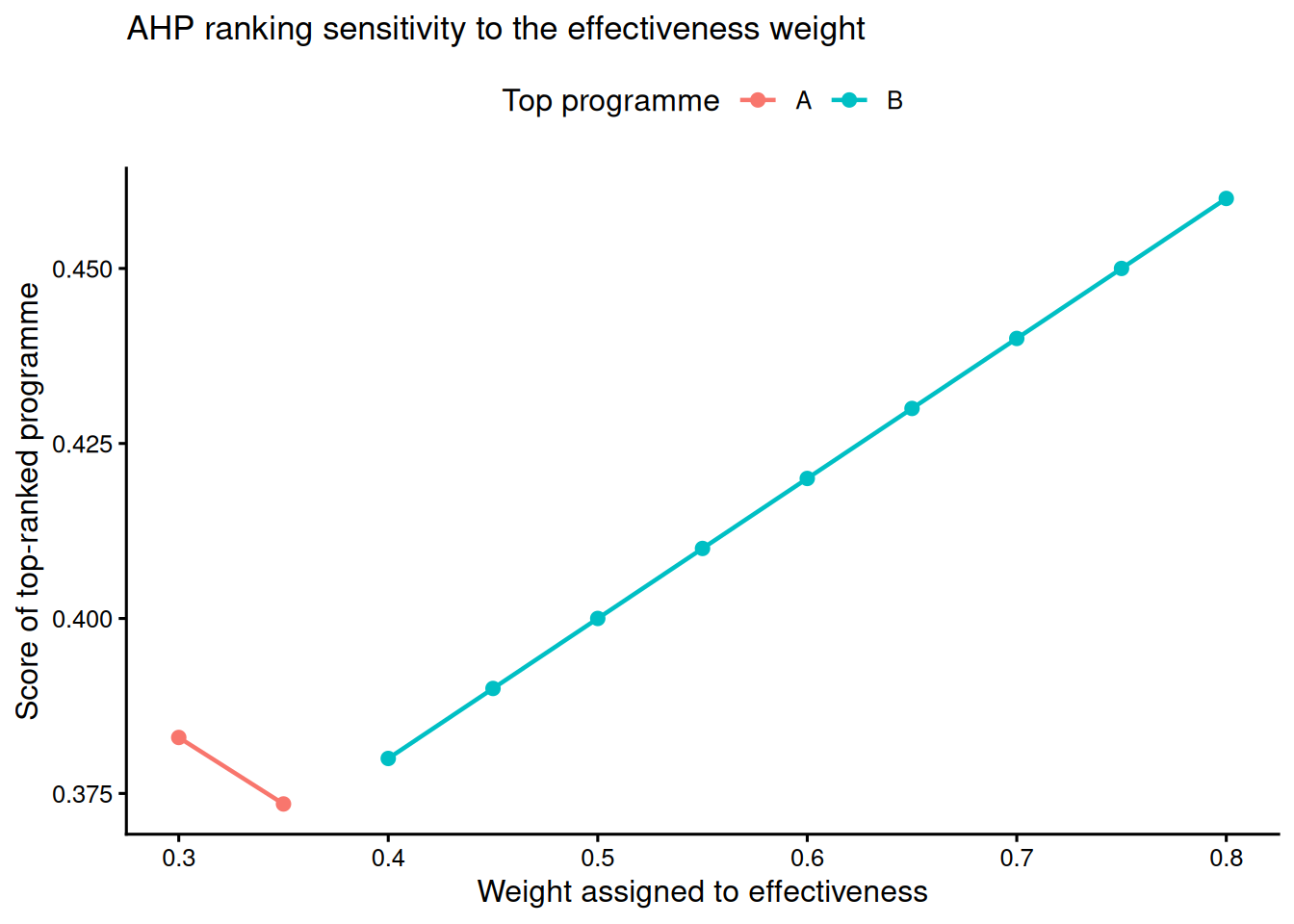
Sensitivity analysis is essential because MCDM rankings can change when weights or normalisation rules change. Figure 14.1 and Table 14.5 vary the weight placed on effectiveness in the AHP example. This is a better way to communicate robustness than presenting a ranking as if it were fixed by the data alone.
The sensitivity loop below perturbs the effectiveness weight and recomputes rankings. In a stakeholder report, repeat this for each contested criterion or use a tornado plot to show rank reversals under +/-20% weight changes.
:::: {.content-visible when-format="html"}
```{webr-r}
#| label: ch14-sensitivity-code-template
#| context: interactive
library(dplyr)
library(purrr)
criteria_names <- c("Cost", "Effectiveness", "Feasibility")
ahp_matrix <- matrix(
c(
1, 1/3, 1/1.5,
3, 1, 2,
1.5, 1/2, 1
),
nrow = 3,
byrow = TRUE,
dimnames = list(criteria_names, criteria_names)
)
eig <- eigen(ahp_matrix)
criteria_weights <- Re(eig$vectors[, 1])
criteria_weights <- criteria_weights / sum(criteria_weights)
names(criteria_weights) <- criteria_names
programme_scores <- tibble(
Programme = c("A", "B", "C"),
Cost = c(0.50, 0.30, 0.20),
Effectiveness = c(0.25, 0.50, 0.25),
Feasibility = c(0.40, 0.30, 0.30)
)
sensitivity_results <- purrr::map_dfr(seq(0.30, 0.80, by = 0.05), function(eff_weight) {
remaining <- 1 - eff_weight
cost_weight <- remaining * (criteria_weights["Cost"] /
(criteria_weights["Cost"] + criteria_weights["Feasibility"]))
feas_weight <- remaining * (criteria_weights["Feasibility"] /
(criteria_weights["Cost"] + criteria_weights["Feasibility"]))
scores <- programme_scores |>
transmute(
Programme,
Score = Cost * cost_weight +
Effectiveness * eff_weight +
Feasibility * feas_weight
) |>
arrange(desc(Score))
tibble(
effectiveness_weight = eff_weight,
top_programme = scores$Programme[1],
ranking = paste(scores$Programme, collapse = " > ")
)
})
sensitivity_results
```
::::
:::: {.content-visible unless-format="html"}
```{r}
#| eval: false
#| label: ch14-sensitivity-code-template-pdf
sensitivity_results <- purrr::map_dfr(seq(0.30, 0.80, by = 0.05), function(eff_weight) {
remaining <- 1 - eff_weight
cost_weight <- remaining * (criteria_weights["Cost"] /
(criteria_weights["Cost"] + criteria_weights["Feasibility"]))
feas_weight <- remaining * (criteria_weights["Feasibility"] /
(criteria_weights["Cost"] + criteria_weights["Feasibility"]))
scores <- programme_scores |>
transmute(
Programme,
Score = Cost * cost_weight +
Effectiveness * eff_weight +
Feasibility * feas_weight
) |>
arrange(desc(Score))
tibble(
effectiveness_weight = eff_weight,
top_programme = scores$Programme[1],
ranking = paste(scores$Programme, collapse = " > ")
)
})
```
::::
```{r}
#| label: ch14-sensitivity-figure
#| echo: false
#| fig-cap: "Figure 14.1: Sensitivity of the AHP top-ranked programme to the effectiveness weight."
#| alt: "Sensitivity of the AHP top-ranked programme to the effectiveness weight."
sensitivity_plot
```
For applied decision reports, a tornado plot can extend this idea by varying each criterion weight by a fixed amount, such as +/-20%, and showing whether the top-ranked alternative changes. That display is often more comprehensive than a single-weight sweep when several criteria are contested.
```{r}
#| label: ch14-sensitivity-table
#| echo: false
#| results: asis
smallsamplelab_apa_table(
"14.5",
"AHP ranking sensitivity as the effectiveness weight changes",
sensitivity_display,
note = "The ranking is stable when Programme B remains first across plausible effectiveness weights. If the top programme changes, stakeholders should discuss whether the weight range is realistic.",
align = c("r", "l", "l")
)
```
### Key Takeaways
MCDM methods help structure decisions with multiple criteria and few alternatives. AHP is useful when pairwise judgements are central. TOPSIS and VIKOR are useful when alternatives can be compared against ideal and compromise profiles. These methods complement statistical inference but do not replace it. Good MCDM reporting makes the judgement calls visible: criteria, scores, weights, normalisation, aggregation, consistency, and sensitivity all need to be shown.
### Self-Assessment Quiz
```{r}
#| echo: false
#| results: asis
source(normalizePath(file.path(dirname(knitr::current_input(dir = TRUE)), "..", "R", "quiz_helpers.R"), mustWork = TRUE))
smallsamplelab_render_quiz(list(
list(
prompt = "When are MCDM methods most appropriate?",
options = c("When the goal is hypothesis testing", "When a small set of alternatives must be ranked using multiple criteria", "When there is only one outcome variable", "When p-values are required"),
answer = 2L,
explanation = "MCDM methods support ranking and selection decisions across multiple criteria. They are decision tools, not hypothesis tests."
),
list(
prompt = "What does AHP's consistency ratio evaluate?",
options = c("Whether residuals are normally distributed", "Whether pairwise judgements are coherent enough to use", "Whether the sample size is large", "Whether every criterion has equal weight"),
answer = 2L,
explanation = "The consistency ratio checks whether pairwise comparisons are logically coherent. High inconsistency means the judgements should be revisited."
),
list(
prompt = "In TOPSIS, what does a larger closeness coefficient mean?",
options = c("The alternative is closer to the ideal and farther from the negative ideal", "The p-value is smaller", "The criterion is less important", "The alternative has a larger sample size"),
answer = 1L,
explanation = "TOPSIS ranks alternatives by relative closeness to the ideal solution. Larger coefficients indicate more preferred alternatives under the chosen weights and normalisation."
),
list(
prompt = "Why must cost criteria often be transformed before TOPSIS?",
options = c("TOPSIS cannot use numbers below zero", "TOPSIS assumes larger criterion values are better", "Cost is always irrelevant", "It is required for statistical significance"),
answer = 2L,
explanation = "TOPSIS treats larger values as preferable. Cost must therefore be converted so that lower cost becomes a higher benefit score."
),
list(
prompt = "Why is sensitivity analysis essential in MCDM?",
options = c("It replaces stakeholder judgement", "It shows whether rankings change under plausible weights or inputs", "It computes exact p-values", "It removes the need to state criteria"),
answer = 2L,
explanation = "Rankings can be sensitive to weights and normalisation. Sensitivity analysis shows whether the preferred alternative is robust or depends on a narrow assumption."
)
))
```