Chapter 12: Methods for Sparse Counts and Short Time Series

Learning Objectives

By the end of this chapter, you will be able to recognise when sparse counts and very short time series make standard large-sample modelling fragile, use exact Poisson procedures for small event counts, compare event rates with appropriate uncertainty, construct transparent forecast intervals for short series, and report overdispersion or zero-inflation without overfitting models the data cannot support.

The Challenge of Sparse Counts

Sparse counts occur when events are rare, exposure is limited, or most units have zero events. In those settings, ordinary Poisson regression can produce unstable standard errors, asymptotic tests can be inaccurate, and zero-inflated or negative binomial models may be too parameter-heavy for the available data. The small-sample goal is usually not to build an elaborate model, but to make a defensible comparison, quantify uncertainty, and explain what the data can and cannot support.

Short time series create a parallel problem. With fewer than about 30 observations, classical ARIMA identification is usually underpowered: there are too few data points to estimate autocorrelation structure reliably. Simple trend summaries, residual-bootstrap intervals, and clearly labelled descriptive forecasts are often more honest than a complex model that appears precise only because it is overfit.

Choosing a Sparse-Data Method

Begin with the data structure rather than the model name. A sparse-count analysis is usually trying to answer one of four questions: whether a count differs from a benchmark rate, whether two rates differ, whether count variability is larger than a Poisson model expects, or whether a short sequence supports a cautious forecast. Each question has a different minimum reporting unit.

Situation	Useful starting point	What must be reported
One small count compared with a known exposure-adjusted benchmark	Exact Poisson test	Event count, exposure, benchmark rate, exact CI and two-sided p-value
Two independent sparse event rates	Exact Poisson rate-ratio comparison	Counts and exposures in both groups, rate ratio, exact CI and p-value
Count outcome with variance much larger than the mean	Poisson summary plus quasi-Poisson sensitivity check	Mean, variance, dispersion estimate, coefficient scale and adjusted standard errors
Overdispersed counts with enough information for an extra parameter	Negative binomial sensitivity analysis	Sample size, theta estimate, standard errors and whether the fit is stable
Many zeros in a very small dataset	Descriptive zero-count reporting before any zero-inflated model	Number and proportion of zeros, total events and why a ZIP model is or is not defensible
Short series with fewer than about 15 observations	Descriptive trend and exploratory interval only	Number of time points, trend assumption, resampling unit, seed and bootstrap resamples

This sequence prevents a common small-sample error: fitting the most specialised model first. Exact and descriptive methods usually give the clearest account of the evidence. More complex models are useful only when they answer a question that the simpler summaries cannot answer and when the data contain enough information to estimate the extra parameters.

Exact Poisson Test for a Benchmark Rate

The exact Poisson test compares an observed count with a pre-specified event rate over a known exposure. In the quality-control example, 15 defects were observed across five batches, against a benchmark of two defects per batch. Table 12.1 shows that the observed rate is higher, but the exact interval still includes the target rate.

Table 12.1

Exact Poisson test for the defect-rate benchmark

Quantity	Value
Observed defects	15
Exposure (batches)	5 batches
Observed rate	3.00 defects per batch
Target rate	2.00 defects per batch
Exact p-value	0.113
95% exact CI for rate	1.68 to 4.95

Note. The exact test compares 15 observed defects over five batches with a target rate of two defects per batch.

The exact two-sided p-value is 0.113, so this small trial does not provide strong evidence that the process rate differs from the benchmark of 2.00 defects per batch at alpha = 0.05. The practical warning remains meaningful: the point estimate is 3.00 defects per batch, and the 95% exact CI (1.68 to 4.95) is wide because only 15 events were observed.

Comparing Two Sparse Event Rates

For two independent event counts, compare rates using the event counts and the exposure times together. Table 12.2 shows the raw rates for two trials, and Table 12.3 reports the exact Poisson rate-ratio comparison.

Table 12.2

Adverse event rates by trial

Trial	Events	Patient-days	Rate per patient-day
A	8	50	0.160
B	3	45	0.067

Note. Rates are events divided by patient-days.

Table 12.3

Exact comparison of adverse event rates

Quantity	Value
Rate ratio (A/B)	2.40
95% exact CI	0.58 to 14.05
Exact p-value	0.234

Note. The exact rate-ratio CI is computed on the log scale and back-transformed. With only 11 total events, the log-scale standard error is large, producing a wide interval on the original rate-ratio scale.

Trial A’s observed rate is higher, with an estimated rate ratio of 2.40. The 95% exact CI (0.58 to 14.05) includes 1 and spans more than an order of magnitude, so the result should be framed as imprecise rather than as evidence of a clear difference. Report the raw event counts and exposure times alongside the ratio so readers can assess how much information supports the estimate.

Bootstrap Forecast Intervals for Short Time Series

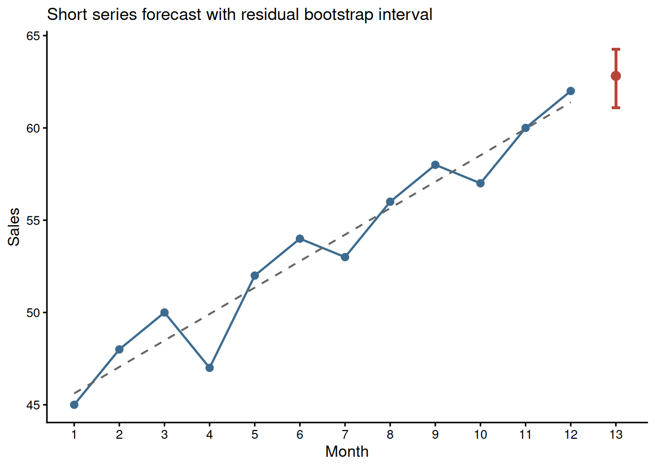
With 12 monthly observations, a simple linear trend can be easier to explain than a fitted ARIMA model. Figure 12.1 shows the observed series, the fitted linear trend, and a residual-bootstrap interval for month 13 (Efron and Tibshirani 1993). Table 12.4 gives the numeric summary.

Figure 12.1: Short monthly sales series with a residual-bootstrap forecast interval for month 13. The interval reflects residual variability around the fitted linear trend but not model-selection or autocorrelation uncertainty.

Table 12.4

Short-series forecast summary

Quantity	Value
Observed months	12
Trend slope	1.43 sales units per month
Month 13 point forecast	62.8
95% residual-bootstrap interval	61.1 to 64.3
Residual autocorrelation check	Ljung-Box p = 0.008

Note. This residual bootstrap resamples model residuals with replacement, adds them to fitted values, refits the trend in each bootstrap sample, and forecasts month 13. It assumes residuals are approximately independent and identically distributed; autocorrelation or structural breaks would require a block bootstrap or state-space approach. The Ljung-Box row is a small-sample screen, not proof of independence.

The forecast is transparent, but it should not be oversold. With only 12 observations, the apparent trend may be sensitive to a few months, and the residual-bootstrap interval is an exploratory forecast band rather than a definitive prediction interval. If the residuals show visible autocorrelation or a structural break, the resampling unit is wrong and this interval should not be used without a time-series-specific bootstrap.

Zero Inflation and Overdispersion

Zero-inflated models estimate both a count process and an extra-zero process, typically adding at least two parameters relative to a standard Poisson model. That can be useful with enough data, such as n = 50 to 100 with clear zero inflation, but in very small samples (n < 30) it often creates more parameters than the dataset can support, leading to unstable estimates or non-convergence (Cameron and Trivedi 2013). A pragmatic first step is to report the proportion of zeros, the mean, and the variance, then decide whether a simple exact or quasi-likelihood approach is adequate.

Table 12.5 summarises the simulated clinic-visit counts. The variance exceeds the mean in both groups, which is a warning sign for overdispersion.

Table 12.5

Clinic visit count summaries by treatment group

Treatment	n	Mean	Variance	Variance/mean	Zero-count cases
Standard	6	2.83	5.37	1.89	1
Enhanced	6	4.83	6.97	1.44	0

Note. When the variance is materially larger than the mean, for example a variance/mean ratio above about 1.5, a standard Poisson model may understate uncertainty. Quasi-Poisson or negative binomial models can provide more realistic standard errors, but with very small samples the dispersion estimate is itself uncertain.

For a fitted Poisson model, the same issue can be checked directly with performance::check_overdispersion(). Use this as a diagnostic prompt rather than a mechanical decision rule; with very small samples, the dispersion estimate can move substantially when one observation changes.

poisson_fit <- glm(visits ~ treatment, family = poisson(), data = visit_data)
performance::check_overdispersion(poisson_fit)

Quasi-Poisson as a Small-Sample Adjustment

A quasi-Poisson model keeps the Poisson mean structure but estimates a dispersion parameter, phi, and inflates standard errors by sqrt(phi). The coefficient estimates remain identical to those from the standard Poisson model; only the standard errors and derived p-values change. When phi > 1, the quasi-Poisson result is more conservative; when phi is close to 1, the two models converge.

Table 12.6

Poisson and quasi-Poisson comparison for clinic visit counts

Model	Log rate ratio	Std. error	p-value	Dispersion estimate
Poisson	0.53	0.31	0.080	1.00 (fixed)
Quasi-Poisson	0.53	0.39	0.206	1.67

Note. The coefficient compares Enhanced with Standard treatment on the log-rate scale. The quasi-Poisson log rate ratio is 0.53, corresponding to a rate ratio of 1.71. The dispersion parameter phi is estimated as the Pearson chi-square statistic divided by residual degrees of freedom; here phi = 1.67, inflating standard errors by about 1.29. p-values are from the Wald test on the log scale. The displayed SE values are rounded; the printed phi is computed from the full Pearson statistic and may not reproduce exactly from rounded SEs.

In this example, the standard Poisson model would make the treatment contrast look more precise than the data justify. The quasi-Poisson result is a useful sensitivity check, but with only 12 observations it should still be reported as exploratory.

Negative Binomial and Zero-Inflated Alternatives

Negative binomial regression is another common response to overdispersed count data. Unlike quasi-Poisson, it specifies a mean-variance relationship and estimates an additional dispersion parameter, usually called theta. That extra parameter can be useful when there is enough information, but with very small samples it is itself unstable. Table 12.7 therefore treats the negative binomial model as a sensitivity check rather than a replacement for the simpler summaries above.

Table 12.7

Negative binomial sensitivity check for clinic visit counts

Quantity	Value
Log rate ratio	0.53
Rate ratio	1.71
Std. error	0.37
p-value	0.146
Theta	7.94

Note. The negative binomial model is fitted with MASS::glm.nb(). With n = 12, the theta estimate is included only as a sensitivity check; the quasi-Poisson and raw count summaries remain central.

The same caution applies more strongly to zero-inflated Poisson models. A zero-inflated model would estimate both the visit-count process and an extra-zero process. In this example there are only 12 observations and only one zero-count case, so a zero-inflated model would add parameters without enough information to estimate them reliably. The defensible report is therefore descriptive: show the zero count, the mean-variance pattern, and the Poisson/quasi-Poisson sensitivity comparison rather than fitting a model that the data cannot support.

Reporting Checklist for Sparse-Count Analyses

State the observed event count and exposure, such as “15 defects across 5 batches.” Report the exact method used, the point estimate, the 95% exact CI, and the two-sided p-value. For rate ratios, give raw counts and exposures for both groups. For resampling procedures, report the random seed and number of bootstrap resamples, such as set.seed(2025) and R = 2000. If using quasi-Poisson, report the dispersion estimate and note that coefficients are unchanged from the Poisson model while standard errors are adjusted. Frame results as exploratory when n < 30 or total events < 20.

Key Takeaways

Sparse counts and short time series reward restraint. Exact Poisson tests provide defensible inference for small event counts and benchmark comparisons, while exact rate-ratio intervals show how quickly uncertainty grows when total events are few. For short series, simple trend models and residual-bootstrap intervals are often more transparent than complex ARIMA models when their assumptions are stated (Hyndman and Athanasopoulos 2021). Zero-inflated and negative binomial models can be appropriate with enough information, but with very small samples researchers should begin with descriptive summaries, dispersion checks, exact tests, and clearly qualified uncertainty.