Chapter 5: Reliability and Measurement Quality for Short Scales

Learning Objectives

By the end of this chapter, you will be able to explain why reliability estimates behave differently in short scales, distinguish alpha, omega, and split-half coefficients, compute the main internal-consistency diagnostics in R, and report measurement quality with appropriate confidence intervals and small-sample caveats.

The Challenge of Short Scales

Many small-sample studies use brief measurement instruments (3–5 items) to reduce respondent burden. Short scales, however, pose challenges for reliability assessment. Classical reliability indices (Cronbach’s alpha, split-half reliability) are attenuated when scales have few items. Moreover, small sample sizes yield imprecise reliability estimates with wide confidence intervals.

Despite these limitations, reliability assessment remains essential. Unreliable measures introduce noise, reducing statistical power and biasing effect estimates. Researchers should report reliability alongside validity evidence and interpret findings cautiously when reliability is low.

Cronbach’s Alpha

Cronbach’s alpha estimates internal consistency by comparing item variances to total scale variance. It assumes that all items measure a single underlying construct and that item true scores contribute equally to the total score, usually described as tau-equivalence. A stricter parallel-items model also requires equal error variances, whereas a congeneric model allows items to have different loadings. Alpha increases with the number of items and the average inter-item correlation.

Assumptions: Items are at least approximately tau-equivalent. Errors are uncorrelated. Continuous or approximately continuous item responses.

When to use: Multi-item scales (3 or more items), desire for simple internal consistency estimate. Interpret cautiously for short scales and with small samples.

Interpreting Alpha in Context

Traditional thresholds (e.g., α ≥ 0.70 for research, α ≥ 0.90 for high-stakes decisions) are heuristic benchmarks, not universal rules (DeVellis and Thorpe 2021):

• Exploratory research / pilot studies: α = 0.60–0.70 acceptable
• Established scales in research: α = 0.70–0.90 expected
• High-stakes decisions: α > 0.90 required
• Very short scales (3 items): α = 0.50–0.65 may be acceptable only when items are conceptually narrow and homogeneous, corrected item-total correlations exceed about 0.30, and the estimate is reported with its confidence interval

The alpha coefficient alone is rarely sufficient for assessing measurement quality. More diagnostic in most small-sample settings are the item-total correlations, which show whether each item contributes meaningfully to the composite; the conceptual coherence of the item set; and the width of the confidence interval around alpha, which reveals how much precision the sample size actually supports.

With n = 36, an alpha of 0.65 has an approximate 95% CI of [0.45, 0.80] under normal-theory assumptions. This wide interval reflects substantial sampling uncertainty: the true population reliability could range from questionable to good. Always report confidence intervals alongside point estimates. The default CI from psych::alpha() is based on an asymptotic standard error, which can be optimistic with small n or non-normal data; when computationally feasible, bootstrap intervals (for example via boot::boot) provide a useful robustness check.

WarningCommon Misconception: “Alpha > 0.70 = Good Scale”

Myth: “If Cronbach’s alpha is above 0.70, my scale is reliable and valid.”

Reality: Alpha can be artificially inflated by redundant items or scale length. High alpha ≠ good measurement.

Demonstration:

library(psych)

# Create a scale with near-duplicate items (bad scale design!)
set.seed(2025)
n <- 30
base_score <- rnorm(n, 50, 10)
redundant_scale <- tibble(
  item1 = base_score,
  item2 = base_score + rnorm(n, 0, 2),
  item3 = base_score + rnorm(n, 0, 2),
  item4 = base_score + rnorm(n, 0, 2)
)

# Compute alpha
invisible(capture.output(
  alpha_result <- suppressWarnings(alpha(redundant_scale))
))

redundant_demo_display <- alpha_result$item.stats %>%
  as.data.frame() %>%
  rownames_to_column("Item") %>%
  transmute(
    Item,
    `Corrected item-total correlation` = round(r.cor, 2)
  )

chapter5_measurement_table(
  "5.1",
  "Corrected item-total correlations for the redundant-item demonstration",
  redundant_demo_display,
  note = paste0(
    "Cronbach's alpha = ",
    formatC(alpha_result$total$raw_alpha, format = "f", digits = 2),
    ". The high value reflects redundancy rather than broad construct coverage."
  ),
  align = c("l", "r")
)

Table 5.1

Corrected item-total correlations for the redundant-item demonstration

Item	Corrected item-total correlation
item1	0.99
item2	0.98
item3	0.98
item4	0.98

Note. Cronbach's alpha = 0.99. The high value reflects redundancy rather than broad construct coverage.

Problems with high-but-meaningless alpha:

1. Redundant items: Asking the same question 10 times inflates alpha but doesn’t improve measurement
2. Alpha increases with # items: 20 poor items can yield α = 0.90 (following the Spearman-Brown relationship)
3. Ignores unidimensionality: Alpha doesn’t test whether items measure one construct or multiple

What to check instead: Ask whether all items contribute meaningfully to the scale through their item-total correlations, whether the mean inter-item correlation falls in a plausible range of about 0.15 to 0.50 (Briggs and Cheek 1986; Clark and Watson 1995), whether the items appear to reflect one coherent factor rather than several unrelated ones, and whether the content still covers the construct broadly enough to be useful. Values below about 0.15 suggest that items do not cohere well, whereas values above about 0.50 often indicate redundancy.

Lesson: Don’t chase alpha > 0.90 by adding redundant items. Better to have α = 0.75 with diverse, non-redundant items than α = 0.95 with near-duplicates.

Example: Cronbach’s Alpha for a Short Scale

We assess the internal consistency of a 3-item service quality scale using the service_quality.csv data.

Rendered Output

Table 5.2

Internal consistency summary for the 3-item service quality scale

Metric	Value
Cronbach's alpha	0.793
Asymptotic standard error	0.060
Bootstrap 95% CI lower bound	0.613
Bootstrap 95% CI upper bound	0.881
Bootstrap resamples	1000.000

Note. The confidence interval is a percentile bootstrap interval over participants. The asymptotic standard error from psych::alpha() is shown for reference but is not used as the primary interval in this small-sample example.

Cell Code

Interpretation: Alpha quantifies the proportion of variance in scale scores attributable to the true score under the working assumptions of the model. Higher alpha indicates stronger internal consistency, but the bootstrap interval shows how uncertain the estimate remains in a small sample. If alpha is below 0.70, consider whether items truly measure a single construct or whether the scale is too heterogeneous. The psych package also reports “alpha if item deleted”, showing how alpha would change if each item were removed; this helps identify problematic items.

Standard Error of Measurement (SEM)

The SEM quantifies measurement precision: how much individual scores vary because of measurement error. In applied reporting, the reliability value is usually an estimate such as \(\hat{\alpha}\) rather than a known population parameter, so the SEM is also an estimate and should be interpreted with the same uncertainty caveat.

Formula: \(\widehat{\text{SEM}} = \text{SD} \times \sqrt{(1 - \hat{\alpha})}\)

Rendered Output

Table 5.3

Standard error of measurement example for a 10-point test

Metric	Value
Scale SD	10.00
Estimated alpha (alpha-hat)	0.75
Estimated SEM	5.00
95% CI half-width	9.80

Cell Code

Interpretation: With \(\widehat{\text{SEM}} = 5\) points, an individual’s true score likely falls within about ±10 points of their observed score under the working reliability estimate. This helps judge whether observed changes are genuine or merely measurement error. In practice, the minimum detectable change is about \(1.96 \times \widehat{\text{SEM}} \times \sqrt{2} \approx 14\) points, so smaller changes could plausibly reflect measurement error alone. Because \(\hat{\alpha}\) is estimated from a small sample, this SEM should be reported as approximate; when individual-level decisions matter, use a confidence band for reliability, or a bootstrap sensitivity check, to show how much the SEM changes across plausible reliability values.

McDonald’s Omega

McDonald’s omega (\(\omega_t\)) is an alternative to alpha that relaxes the tau-equivalence assumption (McDonald 1999). It is computed from a common-factor model and reflects the proportion of variance in scale scores due to common factors. In realistic congeneric settings, omega is often preferred over alpha because it accommodates unequal factor loadings across items (Trizano-Hermosilla and Alvarado 2016).

When to use: Multi-item scales with varying item-factor relationships, when tau-equivalence is questionable, or when reporting alongside alpha for robustness.

Example: McDonald’s Omega

We compute omega for the same 3-item service quality scale.

Rendered Output

Table 5.4

Omega summary for the 3-item service quality scale

Metric	Value
McDonald's omega total	0.803
Cronbach's alpha	0.793
Difference (omega - alpha)	0.010

Note. Omega and alpha are very similar here, which is what we expect for a tightly unidimensional toy example.

Cell Code

Interpretation: The omega() function reports two related indices. \(\omega_t\) (omega total) summarises the proportion of total score variance attributable to all common factors, whereas \(\omega_h\) (omega hierarchical) isolates the variance attributable to a general factor after accounting for group factors. For brief, unidimensional scales, \(\omega_t\) is usually the relevant quantity. \(\omega_h\) is more informative when evaluating multidimensional instruments with a bifactor-like structure.

With a perfectly unidimensional three-item example, some elements of the printed omega() output can look extreme. Values such as omega_h = 1 or max/min = Inf reflect a degenerate single-factor solution with no modeled specific-factor variance. In this setting, they are a consequence of the toy example rather than evidence that the computation failed.

Split-Half Reliability

Split-half reliability divides a scale into two halves, computes the correlation between half-scale scores, and adjusts using the Spearman–Brown formula to estimate reliability of the full scale. The adjustment is \(r_{SB} = \frac{2r_{half}}{1 + r_{half}}\), where \(r_{half}\) is the correlation between the two halves. This matters because reliability increases with scale length. With small samples, split-half estimates are imprecise, and different item splits can yield noticeably different values.

When to use: Multi-item scales, desire for alternative reliability estimate, comparison with alpha or omega.

Example: Split-Half Reliability

We compute split-half reliability for the service quality scale and report the Spearman-Brown adjusted estimate.

Rendered Output

Table 5.5

Split-half reliability summary for the service quality scale

Metric	Value
Spearman-Brown adjusted reliability	0.795
Minimum split-half reliability	0.670
Maximum split-half reliability	0.771
Median split-half reliability	0.679

Note. Least favourable split: q2_professionalism versus q1_responsiveness, q3_clarity.

Cell Code

Interpretation: The split-half correlation measures consistency between the two halves. The Spearman–Brown adjustment estimates the reliability of the full scale. This method is less commonly used than alpha but provides a complementary perspective. Because different item splits can yield different results, it is best treated as a robustness check rather than a single definitive reliability estimate.

Worst Split-Half Reliability (Practical Alternative to Revelle’s Beta)

This chapter reports the minimum split-half reliability across all admissible partitions from psych::splitHalf() as a practical stress test. Earlier editions of this text referenced Revelle’s β, a related lower-bound estimate that focuses on the weakest split-half consistency; current psych workflows fold that logic into splitHalf(), so a separate helper is unnecessary. Unlike omega, which is factor-model based, the worst-split value is a stress test of how fragile the item set becomes under the least favourable partition.

Rendered Output

Table 5.6

Worst-case split-half reliability for the service quality scale

Metric	Value
Least favourable split reliability	0.670
Most favourable split reliability	0.771
Least favourable split A	q2_professionalism
Least favourable split B	q1_responsiveness, q3_clarity

Note. This chapter reports the minimum split-half reliability from psych::splitHalf(). Earlier editions referenced Revelle's β, but current psych workflows integrate that lower-bound logic within splitHalf() (here using psych 2.6.3).

Cell Code

Interpretation: The minimum split-half value is typically lower than the Spearman-Brown adjusted estimate because it focuses on the weakest admissible partition. Large gaps between the overall split-half estimate and the minimum split suggest that some item partitions are fragile, meaning the scale could behave inconsistently across subsets of items. With very small samples, these stress-test values can fluctuate; report them alongside alpha and omega and acknowledge the additional uncertainty.

Polychoric Correlations for Ordinal Items

Likert-scale items (e.g., 1–7 ratings) are ordinal, not continuous. Pearson correlations and alpha computed on ordinal data may underestimate reliability. Polychoric correlations estimate the correlation between underlying continuous latent variables, assuming ordinal responses arise from categorising continuous variables.

When items are ordinal and have few response options, polychoric correlations and ordinal alpha may be more accurate. However, stable estimation often requires roughly n = 50–100, depending on the number of response categories and the observed distributions (Olsson 1979). With smaller samples, polychoric solutions may be unstable or fail to converge; in those cases, report Pearson-based alpha and note that ordinal methods were considered but were too uncertain for strong interpretation.

When to use: Ordinal items with few response categories, ideally with samples closer to n ≥ 50–100 when feasible, and when there is a clear need for theoretically appropriate latent-response correlations.

Example: Polychoric Correlations (Conceptual)

We compute polychoric correlations for the service quality items. With n = 36, this example falls below the preferred range for stable polychoric estimation, so the result should be treated as illustrative rather than definitive.

Rendered Output

Table 5.7

Polychoric correlation matrix for the service quality items

Item	q1_responsiveness	q2_professionalism	q3_clarity
q1_responsiveness	1.000	0.643	0.666
q2_professionalism	0.643	1.000	0.519
q3_clarity	0.666	0.519	1.000

Note. Alpha based on the polychoric correlation matrix = 0.824.

Cell Code

Interpretation: Polychoric correlations are typically higher than Pearson correlations for ordinal data, so alpha computed from the polychoric matrix may also be higher. However, with small samples these estimates can be unstable or fail to converge. If polychoric and Pearson results are similar, the method choice has little practical impact. If they differ substantially, report both and note that the ordinal estimate is more assumption-sensitive in small samples.

Reporting Reliability with Small Samples

When reporting reliability for small samples and short scales:

• Report Cronbach’s alpha with confidence intervals.
• Consider reporting McDonald’s omega as a robustness check.
• Acknowledge limitations (short scale, small sample, wide CIs).
• Provide item-level descriptive statistics (means, SDs, inter-item correlations).
• Discuss implications for interpretation (e.g., “The modest alpha suggests caution in interpreting scale scores; findings should be replicated with longer instruments”).

Lab Practical 5.1: Refining a Workplace Resilience Scale

Context: An organizational psychologist developed a 6-item Workplace Resilience Scale (WRS) to measure employees’ ability to cope with job stress. After piloting the scale with 22 employees, the researcher wants to evaluate internal consistency and decide whether to drop any items to improve reliability. This walkthrough demonstrates item analysis, alpha calculation, and item-deletion decisions.

Learning Goals:

• Compute Cronbach’s alpha for a multi-item scale
• Examine item-total correlations to identify weak items
• Assess the impact of dropping items on reliability
• Make evidence-based decisions about scale refinement
• Understand context-dependent alpha thresholds

Step 1: Load and Explore the Data

Rendered Output

Table 5.8

Item descriptive statistics for the Workplace Resilience Scale pilot

Item	Mean	SD
WRS1	4.00	0.76
WRS2	3.27	0.63
WRS3	4.64	0.49
WRS4	2.14	0.99
WRS5	3.64	0.49
WRS6	3.27	0.63

Cell Code

Checkpoint: Items have similar means (3–4) and SDs (0.5–1.0), except WRS4 shows a lower mean and higher SD. That pattern suggests it may not align with the rest of the scale and could be weakly keyed or reverse-worded.

Step 2: Compute Cronbach’s Alpha (Full Scale)

Rendered Output

Table 5.9

Full-scale reliability summary for the 6-item WRS pilot

Metric	Value
Raw alpha	0.101
Standardized alpha	0.625
Average inter-item correlation	0.218
Signal-to-noise ratio	1.669

Note. The negative WRS4 item pulls the full-scale estimate down sharply and should be inspected before any deletion decision is made.

Cell Code

Checkpoint: The raw alpha is very low here because one item is working in the opposite direction from the rest of the scale, not because every item is equally weak. The standardised alpha asks the same question after putting items on a common variance scale, the mean inter-item correlation shows how tightly the items move together, and the signal-to-noise ratio summarises how much reliable variance remains once error is considered. The key practical question is whether the “reliability if an item is dropped” table shows a sharp improvement for a specific item, because that pattern usually points to reverse coding or conceptual mismatch rather than to a uniformly poor scale.

Step 3: Examine Item-Total Correlations

Rendered Output

Table 5.10

Item-total statistics for the 6-item WRS pilot

Item	Corrected item-total correlation	Raw item-total correlation	Mean	SD
WRS4	-1.077	-0.981	2.136	0.990
WRS5	0.820	0.751	3.636	0.492
WRS3	0.820	0.751	4.636	0.492
WRS2	0.857	0.805	3.273	0.631
WRS6	0.857	0.805	3.273	0.631
WRS1	0.943	0.809	4.000	0.756

Cell Code

Checkpoint: Look for:

• r.cor: Corrected item-total correlation (item vs. scale without that item). Values < 0.30 indicate weak contribution
• r.drop: Raw item-total correlation (item vs. full scale including that item)

Items with r.cor < 0.30 deserve close review. Here, WRS4 is negatively related to the rest of the scale, which points to either an unrecoded reverse-worded item or a construct mismatch rather than simple low reliability.

Step 4: Assess “Alpha if Item Dropped”

Rendered Output

Table 5.11

Alpha if each WRS item were removed

Item	Alpha if item dropped
WRS4	0.937
WRS3	-0.504
WRS5	-0.504
WRS2	-0.827
WRS6	-0.827
WRS1	-1.129

Cell Code

Checkpoint: Dropping WRS4 produces a very large improvement in alpha, which confirms that it is destabilizing the scale. In practice, the next step is to inspect the item wording and scoring key before deciding whether to delete it or reverse-score it.

Step 5: Recompute Alpha Without WRS4

Rendered Output

Table 5.12

Reliability before and after removing WRS4

Scale	Items	Cronbach's alpha
Full 6-item scale	6	0.101
Refined 5-item scale (WRS4 removed)	5	0.937

Note. Alpha increases by 0.836 after removing the misaligned item.

Cell Code

Checkpoint: The refined 5-item scale has much higher alpha and all remaining items show strong positive item-total correlations. That is a more internally consistent measure, but the jump is so large that it also suggests the remaining items may be quite redundant.

Step 6: Interpret in Context

Follow these guidelines:

• Research/exploratory scales: α ≥ 0.60–0.70 acceptable
• Established scales in research: α ≥ 0.70–0.80 preferred
• High-stakes decisions (clinical, personnel): α ≥ 0.80–0.90 required
• Short scales (3–5 items): Expect alpha to run about 0.05–0.10 lower than for longer scales with similar item quality

Decision: WRS4 requires immediate inspection because:

1. It has a negative corrected item-total correlation
2. Dropping it increases alpha dramatically
3. The remaining 5-item scale shows high internal consistency

If WRS4 was intentionally reverse-worded, recode it first and then rerun the reliability analysis before making a final deletion decision.

Step 7: Visualise Item Performance

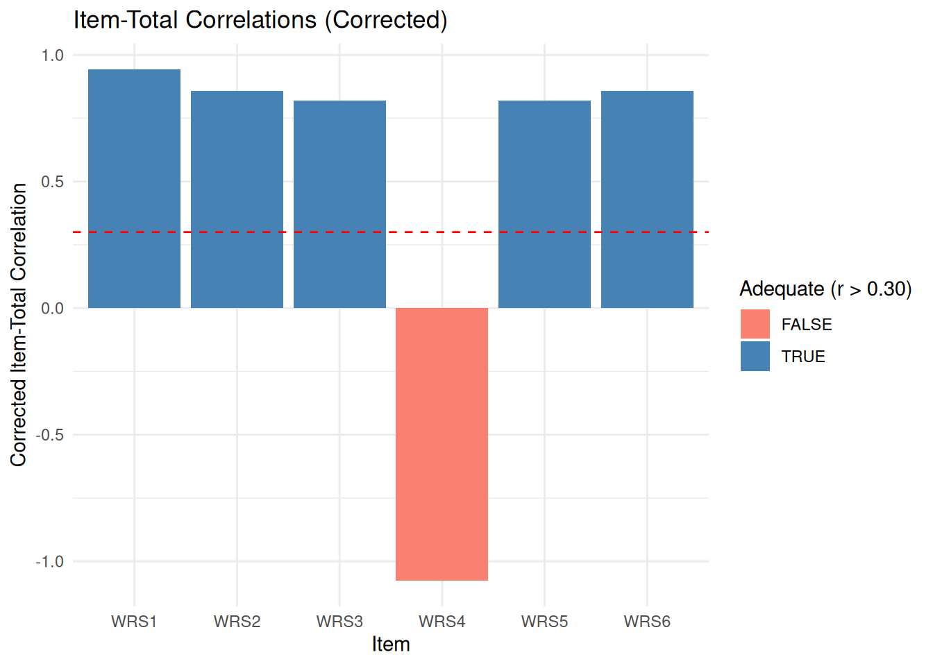
Figure 5.1 shows the corrected item-total correlations for the pilot Workplace Resilience Scale. The dashed reference line marks the usual review threshold of about 0.30, making it easy to see why WRS4 demands immediate follow-up.

Rendered Output

Figure 5.1: Corrected item-total correlations for the pilot Workplace Resilience Scale.

Cell Code

Checkpoint: The plot clearly shows that WRS4 falls well below the acceptable range and in fact moves in the opposite direction from the other items.

Step 8: Report the Results

“The 6-item Workplace Resilience Scale was piloted with 22 employees. Initial reliability analysis suggested severe internal-consistency problems (raw alpha = 0.10), driven by WRS4, which showed a negative corrected item-total correlation (r = -0.98). Removing that item increased alpha to 0.94, indicating that the remaining five items were highly consistent. Before deleting WRS4 permanently, the researcher should verify whether it was intentionally reverse-worded and therefore requires reverse scoring rather than omission. Future validation should use a larger sample and include test-retest reliability.”

Discussion Questions:

1. Why is item-total correlation more informative than item mean or SD? Item-total correlation shows how well an item captures the same construct as the rest of the scale. An item can have a reasonable mean and standard deviation yet still dilute reliability if it does not move with the other items.
2. What if two items both have r.cor < 0.30? Review them one at a time rather than dropping both immediately. Recompute alpha after each change and check whether either item is reverse-worded, badly phrased, or intentionally measuring a distinct facet that the scale still needs.
3. Should you always maximise alpha by dropping items? No. Dropping items can improve internal consistency while also narrowing content coverage too far. In many applied settings, an alpha around 0.70 with broader construct coverage is preferable to a higher alpha achieved by keeping only a few overly redundant items.
4. How does sample size affect these decisions? Small samples make item-total correlations and alpha estimates unstable, so item decisions should remain tentative when n is very limited. Strong deletion decisions are best revisited once a larger validation sample is available.

Extension: Reverse-score WRS4 if its wording is intentionally opposite in direction, then compare the recoded solution with the deletion approach. You can also compute split-half reliability or omega to assess whether the remaining items behave as a coherent short scale.

Key Takeaways

Cronbach’s alpha, McDonald’s omega, and split-half estimates each provide useful but incomplete views of internal consistency. Short scales naturally produce lower coefficients than longer scales, and small samples make all of those estimates more uncertain, which is why confidence intervals and item-level diagnostics matter as much as the point estimate itself. Reliability should therefore be reported transparently, interpreted alongside content coverage and dimensionality, and treated as one part of measurement quality rather than a single threshold to clear.

---

Self-Assessment Quiz

Test your understanding of reliability and measurement quality from Chapter 5.

Question 1. Cronbach’s alpha measures:

Whether data are normally distributedInternal consistency—how closely related a set of items areTest-retest reliabilityInter-rater agreement

Explanation.

Cronbach’s alpha quantifies internal consistency by comparing item variances to total scale variance. It indicates whether items measure a common construct. The chapter states: “Cronbach’s alpha estimates internal consistency by comparing item variances to total scale variance.”

Question 2. What is the main limitation of Cronbach’s alpha?

It requires n>1,000It assumes tau-equivalence (equal factor loadings across items)It cannot be calculated for short scalesIt is always too high

Explanation.

Alpha assumes all items contribute equally to the construct (tau-equivalence). When items have varying loadings, alpha may underestimate reliability. McDonald’s omega relaxes this assumption. The chapter explicitly notes alpha “assumes that all items measure a single underlying construct with equal factor loadings (tau-equivalent model).”

Question 3. A 3-item scale has α=0.55 with n=25. Is this acceptable?

No—alpha must always exceed 0.70Possibly—short scales naturally have lower alpha; consider context, item-total correlations, and CIYes—always acceptableNo—the scale must be discarded

Explanation.

Alpha depends on scale length; 3-item scales often yield α=0.50-0.65 even when internally consistent. Check: (1) item-total correlations (all >0.30?), (2) alpha’s 95% CI (precision), (3) conceptual coherence. For exploratory work, α=0.55 may be acceptable. This reflects the chapter’s nuanced guidance about context-dependent thresholds rather than rigid cutoffs.

Question 4. McDonald’s omega is preferred over alpha when:

Items have equal factor loadingsItems have varying factor loadings (not tau-equivalent)Sample size exceeds 500Data are categorical

Explanation.

Omega (ω_total) allows items to have different factor loadings, providing a more accurate reliability estimate when tau-equivalence does not hold. The chapter states: “McDonald’s omega (ωₜ) is an alternative to alpha that relaxes the tau-equivalence assumption.”

Question 5. Item-total correlation measures:

How well an item correlates with the total scale score (excluding that item)Test-retest stabilityThe mean of all itemsSample size adequacy

Explanation.

Corrected item-total correlation indicates how strongly each item relates to the overall scale. Values <0.30 suggest the item measures something different or is poorly worded. The lab practical emphasizes examining item-total correlations as a diagnostic tool.

Question 6. What does “alpha if item deleted” show?

The p-value for each itemHow alpha would change if a specific item were removedThe mean of each itemWhether items are normally distributed

Explanation.

If alpha increases substantially when an item is removed, that item is weakening internal consistency (low correlation with others or measuring a different construct). Consider revising or removing it. This is a standard feature of reliability analysis output used to identify problematic items.

Question 7. Polychoric correlations are used when:

Items are continuous and normally distributedItems are ordinal (e.g., Likert scales) and you want to estimate correlations between underlying continuous latent variablesSample size exceeds 1,000Data have no missing values

Explanation.

Polychoric correlations assume ordinal responses arise from categorising underlying continuous variables. They often yield higher estimates than Pearson correlations for Likert data, but stable estimation often needs samples closer to n = 50–100. The chapter discusses them as theoretically appropriate for ordinal items, while also warning that very small samples can make them unstable.

Question 8. A scale has α=0.72 with n=36. The 95% CI is [0.52, 0.86]. What does this tell us?

Reliability is excellentReliability is moderate, but precision is limited (wide CI) due to small sampleThe scale is unreliableMore items must be added

Explanation.

The point estimate (0.72) suggests acceptable reliability, but the wide CI reflects substantial uncertainty with n=36. The true population alpha could be as low as 0.52 (questionable) or as high as 0.86 (good). The chapter emphasizes that “small samples produce imprecise reliability estimates with wide confidence intervals.”

Question 9. Split-half reliability involves:

Testing participants twiceDividing items into two halves, computing correlation, and applying Spearman-Brown correctionRemoving half the sampleUsing different raters

Explanation.

Split-half reliability divides a scale into two halves (e.g., odd vs even items), correlates the half-scores, then adjusts using the Spearman-Brown formula to estimate full-scale reliability. This is a classic alternative method for assessing reliability mentioned in the learning objectives.

Question 10. A scale shows α=−0.15. What is the most likely cause?

Perfect reliabilityReverse-coded items not properly recoded, or items measuring different constructsSample size too largeNormal distribution

Explanation.

Negative alpha indicates that the average inter-item covariance is negative. This usually means reverse-coded items were not recoded, but it can also occur when the scale combines items tapping opposing constructs. Check the inter-item correlation matrix for negative values before interpreting the scale.

Ayre, Colin, and Andrew J. Scally. 2014. ‘Critical Values for Lawshe’s Content Validity Ratio: Revisiting the Original Methods of Calculation’. Measurement and Evaluation in Counseling and Development 47 (1): 79–86. https://doi.org/10.1177/0748175613513808.

Briggs, Steven R., and Jonathan M. Cheek. 1986. ‘The Role of Factor Analysis in the Development and Evaluation of Personality Scales’. Journal of Personality 54 (1): 106–48.

Buuren, Stef van. 2018. Flexible Imputation of Missing Data. 2nd ed. Boca Raton, FL: Chapman; Hall/CRC.

Cameron, A. Colin, and Pravin K. Trivedi. 2013. Regression Analysis of Count Data. 2nd ed. Cambridge: Cambridge University Press. https://doi.org/10.1017/CBO9781139013567.

Chen, Henian, Patricia Cohen, and Sophie Chen. 2010. ‘How Big Is a Big Odds Ratio? Interpreting the Magnitudes of Odds Ratios in Epidemiological Studies’. Communications in Statistics - Simulation and Computation 39 (4): 860–64. https://doi.org/10.1080/03610911003650383.

Cicchetti, Domenic V. 1994. ‘Guidelines, Criteria, and Rules of Thumb for Evaluating Normed and Standardized Assessment Instruments in Psychology’. Psychological Assessment 6 (4): 284–90. https://doi.org/10.1037/1040-3590.6.4.284.

Clark, Lee Anna, and David Watson. 1995. ‘Constructing Validity: Basic Issues in Objective Scale Development’. Psychological Assessment 7 (3): 309–19.

Cohen, Jacob. 1988. Statistical Power Analysis for the Behavioral Sciences. 2nd ed. Hillsdale, NJ: Lawrence Erlbaum Associates.

Conover, W. J. 1999. Practical Nonparametric Statistics. 3rd ed. New York: John Wiley & Sons.

Costello, Anna B., and Jason Osborne. 2005. ‘Best Practices in Exploratory Factor Analysis: Four Recommendations for Getting the Most from Your Analysis’. Practical Assessment, Research, and Evaluation 10 (1): 1–9. https://doi.org/10.7275/jyj1-4868.

Davison, A. C., and D. V. Hinkley. 1997. Bootstrap Methods and Their Application. Cambridge Series in Statistical and Probabilistic Mathematics. Cambridge: Cambridge University Press.

DeVellis, Robert F., and Carolyn T. Thorpe. 2021. Scale Development: Theory and Applications. 5th ed. Thousand Oaks, CA: SAGE Publications.

Dienes, Zoltan. 2014. ‘Using Bayes to Get the Most Out of Non-Significant Results’. Frontiers in Psychology 5: 781. https://doi.org/10.3389/fpsyg.2014.00781.

Efron, Bradley, and Robert J. Tibshirani. 1993. An Introduction to the Bootstrap. New York, NY: Chapman; Hall/CRC.

Elm, Erik von, Douglas G. Altman, Matthias Egger, Stuart J. Pocock, Peter C. Gøtzsche, and Jan P. Vandenbroucke. 2007. ‘The Strengthening the Reporting of Observational Studies in Epidemiology (STROBE) Statement: Guidelines for Reporting Observational Studies’. PLoS Medicine 4 (10): e296. https://doi.org/10.1371/journal.pmed.0040296.

Fay, Michael P. 2010. ‘Confidence Intervals That Match Fisher’s Exact or Blaker’s Exact Tests’. Biostatistics 11 (2): 373–74. https://doi.org/10.1093/biostatistics/kxp050.

Firth, David. 1993. ‘Bias Reduction of Maximum Likelihood Estimates’. Biometrika 80 (1): 27–38. https://doi.org/10.1093/biomet/80.1.27.

Gelman, Andrew, Daniel Simpson, and Michael Betancourt. 2017. ‘The Prior Can Often Only Be Understood in the Context of the Likelihood’. Entropy 19 (10): 555. https://doi.org/10.3390/e19100555.

Good, Phillip I. 2005. Permutation, Parametric, and Bootstrap Tests of Hypotheses. 3rd ed. New York: Springer.

Graham, John W. 2009. ‘Missing Data Analysis: Making It Work in the Real World’. Annual Review of Psychology 60: 549–76. https://doi.org/10.1146/annurev.psych.58.110405.085530.

Hair, Joseph F., G. Tomas M. Hult, Christian M. Ringle, and Marko Sarstedt. 2017. A Primer on Partial Least Squares Structural Equation Modeling (PLS-SEM). 2nd ed. Thousand Oaks, CA: SAGE Publications.

Harrell, Frank E. 2015. Regression Modeling Strategies: With Applications to Linear Models, Logistic and Ordinal Regression, and Survival Analysis. 2nd ed. Springer Series in Statistics. New York: Springer. https://doi.org/10.1007/978-3-319-19425-7.

Heinze, Georg, and Michael Schemper. 2002. ‘A Solution to the Problem of Separation in Logistic Regression’. Statistics in Medicine 21 (16): 2409–19. https://doi.org/10.1002/sim.1047.

Hodges, Jr., J. L., and E. L. Lehmann. 1963. ‘Estimates of Location Based on Rank Tests’. The Annals of Mathematical Statistics 34 (2): 598–611. https://doi.org/10.1214/aoms/1177704172.

Hoenig, John M., and Dennis M. Heisey. 2001. ‘The Abuse of Power: The Pervasive Fallacy of Power Calculations for Data Analysis’. The American Statistician 55 (1): 19–24.

Hosmer, David W., Stanley Lemeshow, and Rodney X. Sturdivant. 2013. Applied Logistic Regression. 3rd ed. Wiley Series in Probability and Statistics. Hoboken, NJ: John Wiley & Sons. https://doi.org/10.1002/9781118548387.

Hu, Li-tze, and Peter M. Bentler. 1999. ‘Cutoff Criteria for Fit Indexes in Covariance Structure Analysis: Conventional Criteria Versus New Alternatives’. Structural Equation Modeling 6 (1): 1–55. https://doi.org/10.1080/10705519909540118.

Huberty, Carl J., and Stephen Olejnik. 2006. Applied MANOVA and Discriminant Analysis. 2nd ed. Hoboken, NJ: Wiley. https://doi.org/10.1002/047178947X.

Hwang, Ching-Lai, and Kwangsun Yoon. 1981. Multiple Attribute Decision Making: Methods and Applications. Berlin: Springer. https://doi.org/10.1007/978-3-642-48318-9.

Hyndman, Rob J., and George Athanasopoulos. 2021. Forecasting: Principles and Practice. 3rd ed. Melbourne, Australia: OTexts. https://otexts.com/fpp3/.

Koo, Terry K., and Mae Y. Li. 2016. ‘A Guideline of Selecting and Reporting Intraclass Correlation Coefficients for Reliability Research’. Journal of Chiropractic Medicine 15 (2): 155–63. https://doi.org/10.1016/j.jcm.2016.02.012.

Kraft, Matthew A. 2020. ‘Interpreting Effect Sizes of Education Interventions’. Educational Researcher 49 (4): 241–53. https://doi.org/10.3102/0013189X20912798.

Lakens, Daniël. 2013. ‘Calculating and Reporting Effect Sizes to Facilitate Cumulative Science: A Practical Primer for t-Tests and ANOVAs’. Frontiers in Psychology 4: 863. https://doi.org/10.3389/fpsyg.2013.00863.

Lakens, Daniël, Anne M. Scheel, and Peder M. Isager. 2018. ‘Equivalence Testing for Psychological Research: A Tutorial’. Advances in Methods and Practices in Psychological Science 1 (2): 259–69. https://doi.org/10.1177/2515245918770963.

Lawshe, Charles H. 1975. ‘A Quantitative Approach to Content Validity’. Personnel Psychology 28 (4): 563–75. https://doi.org/10.1111/j.1744-6570.1975.tb01393.x.

Lipsey, Mark W., and David B. Wilson. 1993. ‘The Efficacy of Psychological, Educational, and Behavioural Treatment: Confirmation from Meta-Analysis’. American Psychologist 48 (12): 1181–1209. https://doi.org/10.1037/0003-066X.48.12.1181.

Little, Roderick J. A. 1988. ‘A Test of Missing Completely at Random for Multivariate Data with Missing Values’. Journal of the American Statistical Association 83 (404): 1198–1202. https://doi.org/10.1080/01621459.1988.10478722.

MacKinnon, David P., Jennifer L. Krull, and Chondra M. Lockwood. 2000. ‘Equivalence of the Mediation, Confounding and Suppression Effect’. Prevention Science 1 (4): 173–81.

Mair, Patrick, and Rand R. Wilcox. 2020. ‘Robust Statistical Methods in r Using the WRS2 Package’. Behavior Research Methods 52 (2): 464–88. https://doi.org/10.3758/s13428-019-01246-w.

Mann, Henry B., and Donald R. Whitney. 1947. ‘On a Test of Whether One of Two Random Variables Is Stochastically Larger Than the Other’. The Annals of Mathematical Statistics 18 (1): 50–60. https://doi.org/10.1214/aoms/1177730491.

McDonald, Roderick P. 1999. Test Theory: A Unified Treatment. Mahwah, NJ: Lawrence Erlbaum Associates.

Morey, Richard D., and Jeffrey N. Rouder. 2011. ‘Bayes Factor Approaches for Testing Interval Null Hypotheses’. Psychological Methods 16 (4): 406–19. https://doi.org/10.1037/a0024377.

Nielsen, Jakob. 1993. Usability Engineering. San Francisco, CA: Morgan Kaufmann.

Olsson, Ulf. 1979. ‘Maximum Likelihood Estimation of the Polychoric Correlation Coefficient’. Psychometrika 44 (4): 443–60.

Opricovic, Serafim, and Gwo-Hshiung Tzeng. 2004. ‘Compromise Solution by MCDM Methods: A Comparative Analysis of VIKOR and TOPSIS’. European Journal of Operational Research 156 (2): 445–55. https://doi.org/10.1016/S0377-2217(03)00020-1.

Page, Matthew J., Joanne E. McKenzie, Patrick M. Bossuyt, Isabelle Boutron, Tammy C. Hoffmann, Cynthia D. Mulrow, Larissa Shamseer, et al. 2021. ‘The PRISMA 2020 Statement: An Updated Guideline for Reporting Systematic Reviews’. BMJ 372: n71. https://doi.org/10.1136/bmj.n71.

R Core Team. 2026. R: A Language and Environment for Statistical Computing. Vienna, Austria: R Foundation for Statistical Computing. https://www.R-project.org/.

Rubin, Donald B. 1987. Multiple Imputation for Nonresponse in Surveys. New York, NY: Wiley.

Saaty, Thomas L. 1980. The Analytic Hierarchy Process. New York, NY: McGraw-Hill.

Schulz, Kenneth F., Douglas G. Altman, and David Moher. 2010. ‘CONSORT 2010 Statement: Updated Guidelines for Reporting Parallel Group Randomised Trials’. BMJ 340: c332. https://doi.org/10.1136/bmj.c332.

Shan, Guogen. 2018. Exact Statistical Inference for Categorical Data. London: Academic Press.

Sterne, Jonathan A. C., Ian R. White, John B. Carlin, Michael Spratt, Patrick Royston, Michael G. Kenward, Angela M. Wood, and James R. Carpenter. 2009. ‘Multiple Imputation for Missing Data in Epidemiological and Clinical Research: Potential and Pitfalls’. BMJ 338: b2393. https://doi.org/10.1136/bmj.b2393.

Teare, M. Dawn, Munyaradzi Dimairo, Neil Shephard, Amanda Hayman, Amy Whitehead, and Stephen J. Walters. 2014. ‘Sample Size Requirements to Estimate Key Design Parameters from External Pilot Randomised Controlled Trials: A Simulation Study’. Trials 15: 264. https://doi.org/10.1186/1745-6215-15-264.

Tomczak, Maciej, and Ewa Tomczak. 2014. ‘The Need to Report Effect Size Estimates Revisited: An Overview of Some Recommended Measures of Effect Size’. Trends in Sport Sciences 21 (1): 19–25.

Trizano-Hermosilla, Italo, and Jose M. Alvarado. 2016. ‘Best Alternatives to Cronbach’s Alpha Reliability in Realistic Conditions: Congeneric and Asymmetrical Measurements’. Frontiers in Psychology 7: 769. https://doi.org/10.3389/fpsyg.2016.00769.

Van de Schoot, Rens, and Milica Miočević. 2020. Small Sample Size Solutions: A Guide for Applied Researchers and Practitioners. London: Routledge.

Vehtari, Aki, Andrew Gelman, and Jonah Gabry. 2017. ‘Practical Bayesian Model Evaluation Using Leave-One-Out Cross-Validation and WAIC’. Statistics and Computing 27 (5): 1413–32. https://doi.org/10.1007/s11222-016-9696-4.

Wagenmakers, Eric-Jan, Jonathon Love, Maarten Marsman, Tahira Jamil, Alexander Ly, Josine Verhagen, Ravi Selker, et al. 2018. ‘Bayesian Inference for Psychology. Part II: Example Applications with JASP’. Psychonomic Bulletin & Review 25 (1): 58–76. https://doi.org/10.3758/s13423-017-1323-7.

White, Ian R., Patrick Royston, and Angela M. Wood. 2011. ‘Multiple Imputation Using Chained Equations: Issues and Guidance for Practice’. Statistics in Medicine 30 (4): 377–99. https://doi.org/10.1002/sim.4067.