```{r}
#| include: false
suppressPackageStartupMessages(library(dplyr))
suppressPackageStartupMessages(library(ggplot2))
suppressPackageStartupMessages(library(knitr))
suppressPackageStartupMessages(library(htmltools))
suppressPackageStartupMessages(library(tibble))
chapter3_sampling_emit_table_styles <- function() {
if (isTRUE(getOption("smallsamplelab.chapter3_sampling_table_styles_emitted"))) {
return(invisible(NULL))
}
cat(
"<style>
.chapter3-sampling-apa-table-block {
font-family: 'Times New Roman', Georgia, serif;
color: #111;
max-width: 52rem;
margin-bottom: 1rem;
}
.chapter3-sampling-apa-table-number {
margin: 0 0 0.1rem 0;
font-weight: 700;
}
.chapter3-sampling-apa-table-title {
margin: 0 0 0.55rem 0;
font-style: italic;
}
.chapter3-sampling-apa-table {
width: 100%;
border-collapse: collapse;
font-size: 0.98rem;
line-height: 1.35;
}
.chapter3-sampling-apa-table th,
.chapter3-sampling-apa-table td {
padding: 0.35rem 0.5rem;
border-left: none !important;
border-right: none !important;
background: transparent !important;
vertical-align: top;
}
.chapter3-sampling-apa-table thead th {
border-top: 2px solid #000;
border-bottom: 1px solid #000;
font-weight: 600;
}
.chapter3-sampling-apa-table tbody tr:last-child td {
border-bottom: 2px solid #000;
}
.chapter3-sampling-apa-table-note {
margin: 0.45rem 0 0 0;
font-size: 0.92rem;
line-height: 1.35;
}
</style>\n",
sep = ""
)
options(smallsamplelab.chapter3_sampling_table_styles_emitted = TRUE)
invisible(NULL)
}
chapter3_sampling_html_table <- function(number, title, data, note = NULL,
align = rep("l", ncol(data)),
col.names = names(data)) {
chapter3_sampling_emit_table_styles()
table_view <- tags$div(
class = "chapter3-sampling-apa-table-block",
tags$p(class = "chapter3-sampling-apa-table-number", paste("Table", number)),
tags$p(class = "chapter3-sampling-apa-table-title", title),
HTML(
knitr::kable(
data,
format = "html",
align = align,
col.names = col.names,
escape = FALSE,
table.attr = "class='chapter3-sampling-apa-table'"
)
),
if (!is.null(note)) {
tags$p(class = "chapter3-sampling-apa-table-note", HTML(note))
}
)
htmltools::html_print(table_view)
}
```
# Chapter 3: Sampling Strategies for Small Studies
Sampling in small studies is less about chasing generic sample-size rules and more about matching design ambitions to the population you can realistically access. This chapter explains how to choose between probability and non-probability sampling, how to justify feasible sample sizes honestly, and how to think about power, precision, and adaptation when recruitment is constrained from the outset.
### Learning Objectives
By the end of this chapter, you will be able to explain the trade-offs between probability and purposive sampling, select appropriate sampling methods given realistic resource and population constraints, calculate minimum detectable effects for a planned sample size, and justify sample sizes transparently in research proposals and reports.
### The Tension Between Ideal and Feasible Sample Sizes
Many introductory guides rely on heuristics such as *n* of 30 or more per group for simple group comparisons or 10-15 events per predictor in regression. These are rough planning rules, not universal thresholds. In practice, resource constraints, rare populations, and ethical considerations often make even those targets unattainable. Rather than abandoning research in such contexts, we should adopt methods suited to smaller samples and report findings with appropriate caveats.
Transparent reporting of sampling rationale, achieved sample size, and power or precision estimates helps readers judge the strength of evidence. Researchers should distinguish between studies designed to test specific hypotheses (which require adequate power) and exploratory studies that generate hypotheses or provide preliminary effect estimates (which can proceed with modest samples).
### Probability Sampling with Small Samples
Probability sampling (simple random sampling, stratified sampling, cluster sampling) ensures that every unit has a known, non-zero probability of selection. This supports generalisation to the target population and enables design-based inference. However, probability sampling requires a sampling frame and may be logistically complex or expensive.
With small samples, probability sampling can still be valuable, but estimates will have wide confidence intervals. Stratified sampling, which divides the population into strata and samples proportionally or disproportionately from each, can improve precision by ensuring representation of key subgroups. Probability sampling is most appropriate when a sampling frame is accessible, generalisability to the target population is a genuine aim, and resources permit systematic random selection even if the total sample remains modest.
### Sequential and Adaptive Sampling
When recruitment is costly or uncertain, sequential designs allow researchers to review interim results and decide whether to continue sampling. For example, you might pre-specify that recruitment will proceed in waves of five participants, stopping early if credible intervals for the primary outcome are sufficiently narrow or if feasibility metrics (e.g., consent rates) fall below thresholds. Adaptive sampling can also target underrepresented strata after an initial wave, improving balance without committing to a large upfront sample. To keep this defensible, decision rules should be set in advance, error control should be maintained with methods appropriate for small *n*, and any adaptations should be documented transparently so readers can see how the design evolved.
Sequential or response-adaptive sampling is especially valuable in rare populations, where pausing after each wave prevents over-committing resources if early data already provide actionable evidence.
### Example: Stratified Sampling Calculation
Suppose we are surveying employees in a small organisation with 120 total staff: 60 in Department A, 40 in Department B, 20 in Department C. We can afford to survey 30 employees. Proportional stratified sampling ensures each department is represented in proportion to its size.
:::: {.content-visible when-format="html"}
```{webr-r}
#| label: chapter3-sampling-table-helpers
#| context: setup
#| include: false
#| echo: false
library(dplyr)
library(knitr)
library(htmltools)
library(tibble)
chapter3_sampling_emit_table_styles <- function() {
if (isTRUE(getOption("smallsamplelab.chapter3_sampling_table_styles_emitted"))) {
return(invisible(NULL))
}
cat(
"<style>
.chapter3-sampling-apa-table-block {
font-family: 'Times New Roman', Georgia, serif;
color: #111;
max-width: 52rem;
margin-bottom: 1rem;
}
.chapter3-sampling-apa-table-number {
margin: 0 0 0.1rem 0;
font-weight: 700;
}
.chapter3-sampling-apa-table-title {
margin: 0 0 0.55rem 0;
font-style: italic;
}
.chapter3-sampling-apa-table {
width: 100%;
border-collapse: collapse;
font-size: 0.98rem;
line-height: 1.35;
}
.chapter3-sampling-apa-table th,
.chapter3-sampling-apa-table td {
padding: 0.35rem 0.5rem;
border-left: none !important;
border-right: none !important;
background: transparent !important;
vertical-align: top;
}
.chapter3-sampling-apa-table thead th {
border-top: 2px solid #000;
border-bottom: 1px solid #000;
font-weight: 600;
}
.chapter3-sampling-apa-table tbody tr:last-child td {
border-bottom: 2px solid #000;
}
.chapter3-sampling-apa-table-note {
margin: 0.45rem 0 0 0;
font-size: 0.92rem;
line-height: 1.35;
}
</style>\n",
sep = ""
)
options(smallsamplelab.chapter3_sampling_table_styles_emitted = TRUE)
invisible(NULL)
}
chapter3_sampling_html_table <- function(number, title, data, note = NULL,
align = rep("l", ncol(data)),
col.names = names(data)) {
chapter3_sampling_emit_table_styles()
table_view <- tags$div(
class = "chapter3-sampling-apa-table-block",
tags$p(class = "chapter3-sampling-apa-table-number", paste("Table", number)),
tags$p(class = "chapter3-sampling-apa-table-title", title),
HTML(
knitr::kable(
data,
format = "html",
align = align,
col.names = col.names,
escape = FALSE,
table.attr = "class='chapter3-sampling-apa-table'"
)
),
if (!is.null(note)) {
tags$p(class = "chapter3-sampling-apa-table-note", HTML(note))
}
)
htmltools::html_print(table_view)
}
```
::::
:::: {.content-visible when-format="html"}
::::: {.panel-tabset group="part-b-data-collection-chapter-3-sampling-strategies-for-small-studies-cell-1"}
#### Output
```{webr-r}
#| label: part-b-chunk-01-output
#| context: output
# Population strata
strata <- tibble(
Department = c("A", "B", "C"),
Population_N = c(60, 40, 20),
Proportion = Population_N / sum(Population_N)
)
# Total sample size
total_sample <- 30
# Allocate sample proportionally
strata <- strata %>%
mutate(
Sample_n = round(Proportion * total_sample),
Sampling_Fraction = Sample_n / Population_N
)
strata_display_table <- strata %>%
mutate(
Proportion = sprintf("%.3f", Proportion),
Sampling_Fraction = sprintf("%.2f", Sampling_Fraction)
)
chapter3_sampling_html_table(
"3.1",
"Proportional stratified sampling allocation",
strata_display_table,
note = "<em>Note.</em> The rounded allocation preserves the total sample size of 30 and gives each department the same 25% sampling fraction.",
align = c("l", "r", "r", "r", "r"),
col.names = c("Department", "Population N", "Proportion", "Sample n", "Sampling fraction")
)
```
#### R Code
```{webr-r}
#| label: part-b-chunk-01-code
#| context: interactive
# Population strata
strata <- tibble(
Department = c("A", "B", "C"),
Population_N = c(60, 40, 20),
Proportion = Population_N / sum(Population_N)
)
# Total sample size
total_sample <- 30
# Allocate sample proportionally
strata <- strata %>%
mutate(
Sample_n = round(Proportion * total_sample),
Sampling_Fraction = Sample_n / Population_N
)
strata_display_table <- strata %>%
mutate(
Proportion = sprintf("%.3f", Proportion),
Sampling_Fraction = sprintf("%.2f", Sampling_Fraction)
)
chapter3_sampling_html_table(
"3.1",
"Proportional stratified sampling allocation",
strata_display_table,
note = "<em>Note.</em> The rounded allocation preserves the total sample size of 30 and gives each department the same 25% sampling fraction.",
align = c("l", "r", "r", "r", "r"),
col.names = c("Department", "Population N", "Proportion", "Sample n", "Sampling fraction")
)
```
:::::
::::
:::: {.content-visible unless-format="html"}
```{r}
#| label: part-b-chunk-01
#| results: asis
#| tbl-cap: "Proportional stratified sampling allocation."
# Population strata
strata <- tibble(
Department = c("A", "B", "C"),
Population_N = c(60, 40, 20),
Proportion = Population_N / sum(Population_N)
)
# Total sample size
total_sample <- 30
# Allocate sample proportionally
strata <- strata %>%
mutate(
Sample_n = round(Proportion * total_sample),
Sampling_Fraction = Sample_n / Population_N
)
strata_display_table <- strata %>%
mutate(
Proportion = sprintf("%.3f", Proportion),
Sampling_Fraction = sprintf("%.2f", Sampling_Fraction)
)
knitr::kable(
strata_display_table,
align = c("l", "r", "r", "r", "r"),
col.names = c("Department", "Population N", "Proportion", "Sample n", "Sampling fraction"),
booktabs = TRUE
)
cat(
"\n\n*Note.* The rounded allocation preserves the total sample size of 30 and gives each department the same 25% sampling fraction.\n"
)
```
::::
::: {.callout-note appearance="simple" icon=false}
## Interpretation
Proportional allocation ensures that each department contributes to the sample in proportion to its population size. Department A, being the largest, provides 15 respondents, while Department C, the smallest, provides 5. If employees are then selected randomly within each department, this approach yields unbiased estimates for the overall population. If precision for small strata is a concern, disproportionate allocation (oversampling small strata) can be used, though this requires weighting in analysis.
:::
### Purposive and Convenience Sampling
Purposive (judgmental) sampling selects units based on researcher judgement of their informativeness or representativeness. Convenience sampling selects units that are easily accessible. Neither method supports probabilistic generalisation, but both are common in small-sample research where probability sampling is infeasible.
Findings from purposive or convenience samples should be interpreted cautiously and presented as preliminary or context-specific. Replication in independent samples strengthens confidence. These approaches are most appropriate when no sampling frame is available, the work is exploratory or pilot-focused, the population is rare or hard to reach, or the available resources are tightly constrained.
### Quota Sampling
Quota sampling (a form of purposive sampling) selects units to match known population characteristics (such as age, gender, or occupation distribution). It mimics stratified sampling but without random selection within strata. Quota sampling can improve representativeness compared to convenience sampling, though it remains non-probabilistic. It is most useful when the researcher knows which population characteristics should be balanced but probability sampling is infeasible.
For example, suppose a student satisfaction study can recruit only 30 participants from a programme where the student body is 60% first-year, 25% second-year, and 15% final-year students. A quota plan could recruit 18 first-year, 8 second-year, and 4 final-year students. That improves coverage compared with accepting the first 30 volunteers, but it still does not justify ordinary probability-based confidence intervals unless participants are randomly selected within each quota cell.
| Year group | Population share | Quota for n = 30 |
|---|---:|---:|
| First year | 60% | 18 |
| Second year | 25% | 8 |
| Final year | 15% | 4 |
The report should therefore state the quota variables, the target quotas, the achieved quotas, and the recruitment procedure. Findings should be framed as balanced descriptive evidence rather than population estimates with known sampling error.
Snowball sampling is another non-probability approach for hard-to-reach populations. Initial participants refer other eligible participants, creating a sample through social or professional networks. This can be appropriate for rare populations or sensitive topics, but the findings should be interpreted as network-specific because people outside the referral chains had little or no chance of inclusion.
### Power and Precision with Small Samples
Statistical power is the probability of detecting a true effect of a given size. With small samples, power is limited, meaning that even if a meaningful effect exists, the study may fail to detect it (high Type II error rate). Researchers should conduct power analyses before data collection to understand what effects are detectable given sample size constraints.
If the achieved sample size is smaller than desired, report the minimum detectable effect (MDE): the smallest effect the study can detect with specified power (typically 80%) and alpha (typically 0.05). This helps readers judge whether the study could have detected effects of practical importance.
### Finite Population Correction
When sampling without replacement from a small, known population, the variance of estimates decreases because each sampled unit reduces remaining uncertainty. The finite population correction (FPC) captures that reduction and can lower the required sample size.
In this example, the infinite-population calculation gives a required sample size of 30, but the accessible population is only 120 people. Applying the FPC reduces the required sample size to about 24, as Table 3.2 shows.
:::: {.content-visible when-format="html"}
::::: {.panel-tabset group="part-b-data-collection-chapter-3-sampling-strategies-for-small-studies-cell-2"}
#### Output
```{webr-r}
#| label: part-b-chunk-02-output
#| context: output
# Finite population correction example
n_required_infinite <- 30 # From power analysis
N_population <- 120 # Size of accessible population
n_adjusted <- n_required_infinite /
(1 + (n_required_infinite - 1) / N_population)
fpc_display_table <- tibble(
`Required n (infinite population)` = n_required_infinite,
`Accessible population` = N_population,
`Adjusted n (FPC)` = sprintf("%.2f", n_adjusted),
Reduction = sprintf("%.2f", n_required_infinite - n_adjusted)
)
chapter3_sampling_html_table(
"3.2",
"Finite population correction example",
fpc_display_table,
note = "<em>Note.</em> The adjusted value is shown to two decimals; in practice, required sample sizes are usually rounded up. Because the FPC reflects a reduction in required precision, rounding to the nearest integer (24) rather than up (25) is the conventional choice here.",
align = c("r", "r", "r", "r")
)
```
#### R Code
```{webr-r}
#| label: part-b-chunk-02-code
#| context: interactive
# Finite population correction example
n_required_infinite <- 30 # From power analysis
N_population <- 120 # Size of accessible population
n_adjusted <- n_required_infinite /
(1 + (n_required_infinite - 1) / N_population)
fpc_display_table <- tibble(
`Required n (infinite population)` = n_required_infinite,
`Accessible population` = N_population,
`Adjusted n (FPC)` = sprintf("%.2f", n_adjusted),
Reduction = sprintf("%.2f", n_required_infinite - n_adjusted)
)
chapter3_sampling_html_table(
"3.2",
"Finite population correction example",
fpc_display_table,
note = "<em>Note.</em> The adjusted value is shown to two decimals; in practice, required sample sizes are usually rounded up. Because the FPC reflects a reduction in required precision, rounding to the nearest integer (24) rather than up (25) is the conventional choice here.",
align = c("r", "r", "r", "r")
)
```
:::::
::::
:::: {.content-visible unless-format="html"}
```{r}
#| label: part-b-chunk-02
#| results: asis
#| tbl-cap: "Finite population correction example."
# Finite population correction example
n_required_infinite <- 30 # From power analysis
N_population <- 120 # Size of accessible population
n_adjusted <- n_required_infinite /
(1 + (n_required_infinite - 1) / N_population)
fpc_display_table <- tibble(
`Required n (infinite population)` = n_required_infinite,
`Accessible population` = N_population,
`Adjusted n (FPC)` = sprintf("%.2f", n_adjusted),
Reduction = sprintf("%.2f", n_required_infinite - n_adjusted)
)
knitr::kable(
fpc_display_table,
align = c("r", "r", "r", "r"),
booktabs = TRUE
)
cat(
"\n\n*Note.* The adjusted value is shown to two decimals; in practice, required sample sizes are usually rounded up. Because the FPC reflects a reduction in required precision, rounding to the nearest integer (24) rather than up (25) is the conventional choice here.\n"
)
```
::::
::: {.callout-note appearance="simple" icon=false}
## Interpretation
Sampling without replacement from 120 individuals means that a sample of roughly 24 (instead of 30) achieves the same precision. Always report whether you applied the FPC so readers can replicate the calculation.
:::
### Example: Power Calculation for a Small Study
We plan a study comparing two groups with n = 12 per group. Under a two-sample t-test, the power to detect a medium effect size (Cohen's d = 0.5) is only about 0.22. Reaching 80% power with this design would require sensitivity to a much larger effect, about d = 1.20, as Table 3.3 shows.
:::: {.content-visible when-format="html"}
::::: {.panel-tabset group="part-b-data-collection-chapter-3-sampling-strategies-for-small-studies-cell-3"}
#### Output
```{webr-r}
#| label: part-b-chunk-03-output
#| context: output
# Base R power calculation; setting sd = 1 means delta is on Cohen's d scale.
power_result <- power.t.test(
n = 12,
delta = 0.5,
sd = 1,
sig.level = 0.05,
type = "two.sample",
alternative = "two.sided"
)
# What effect size is detectable with 80% power?
mde_result <- power.t.test(
n = 12,
power = 0.80,
delta = NULL,
sd = 1,
sig.level = 0.05,
type = "two.sample",
alternative = "two.sided"
)
power_display_table <- tibble(
`Per-group n` = 12,
`Target effect (d)` = sprintf("%.2f", 0.5),
`Estimated power` = sprintf("%.2f", power_result$power),
`MDE for 80% power` = sprintf("%.2f", mde_result$delta)
)
chapter3_sampling_html_table(
"3.3",
"Power summary for a two-group small study",
power_display_table,
note = "<em>Note.</em> Setting <code>sd = 1</code> expresses <code>delta</code> on Cohen's <em>d</em> scale.",
align = c("r", "r", "r", "r")
)
```
#### R Code
```{webr-r}
#| label: part-b-chunk-03-code
#| context: interactive
# Base R power calculation; setting sd = 1 means delta is on Cohen's d scale.
power_result <- power.t.test(
n = 12,
delta = 0.5,
sd = 1,
sig.level = 0.05,
type = "two.sample",
alternative = "two.sided"
)
# What effect size is detectable with 80% power?
mde_result <- power.t.test(
n = 12,
power = 0.80,
delta = NULL,
sd = 1,
sig.level = 0.05,
type = "two.sample",
alternative = "two.sided"
)
power_display_table <- tibble(
`Per-group n` = 12,
`Target effect (d)` = sprintf("%.2f", 0.5),
`Estimated power` = sprintf("%.2f", power_result$power),
`MDE for 80% power` = sprintf("%.2f", mde_result$delta)
)
chapter3_sampling_html_table(
"3.3",
"Power summary for a two-group small study",
power_display_table,
note = "<em>Note.</em> Setting <code>sd = 1</code> expresses <code>delta</code> on Cohen's <em>d</em> scale.",
align = c("r", "r", "r", "r")
)
```
:::::
::::
:::: {.content-visible unless-format="html"}
```{r}
#| label: part-b-chunk-03
#| results: asis
#| tbl-cap: "Power summary for a two-group small study."
# Base R power calculation; setting sd = 1 means delta is on Cohen's d scale.
power_result <- power.t.test(
n = 12,
delta = 0.5,
sd = 1,
sig.level = 0.05,
type = "two.sample",
alternative = "two.sided"
)
# What effect size is detectable with 80% power?
mde_result <- power.t.test(
n = 12,
power = 0.80,
delta = NULL,
sd = 1,
sig.level = 0.05,
type = "two.sample",
alternative = "two.sided"
)
power_display_table <- tibble(
`Per-group n` = 12,
`Target effect (d)` = sprintf("%.2f", 0.5),
`Estimated power` = sprintf("%.2f", power_result$power),
`MDE for 80% power` = sprintf("%.2f", mde_result$delta)
)
knitr::kable(
power_display_table,
align = c("r", "r", "r", "r"),
booktabs = TRUE
)
cat(
"\n\n*Note.* Setting `sd = 1` expresses `delta` on Cohen's *d* scale.\n"
)
```
::::
::: {.callout-note appearance="simple" icon=false}
## Interpretation
With 12 participants per group, power to detect a medium effect (d = 0.5) is low, at about 22%. To achieve 80% power, the study would need to be sensitive to a much larger effect (about d = 1.2). This illustrates the limitation of small samples for hypothesis testing. If the true effect is small or medium, the study is underpowered. Researchers should acknowledge this limitation and interpret non-significant results cautiously.
:::
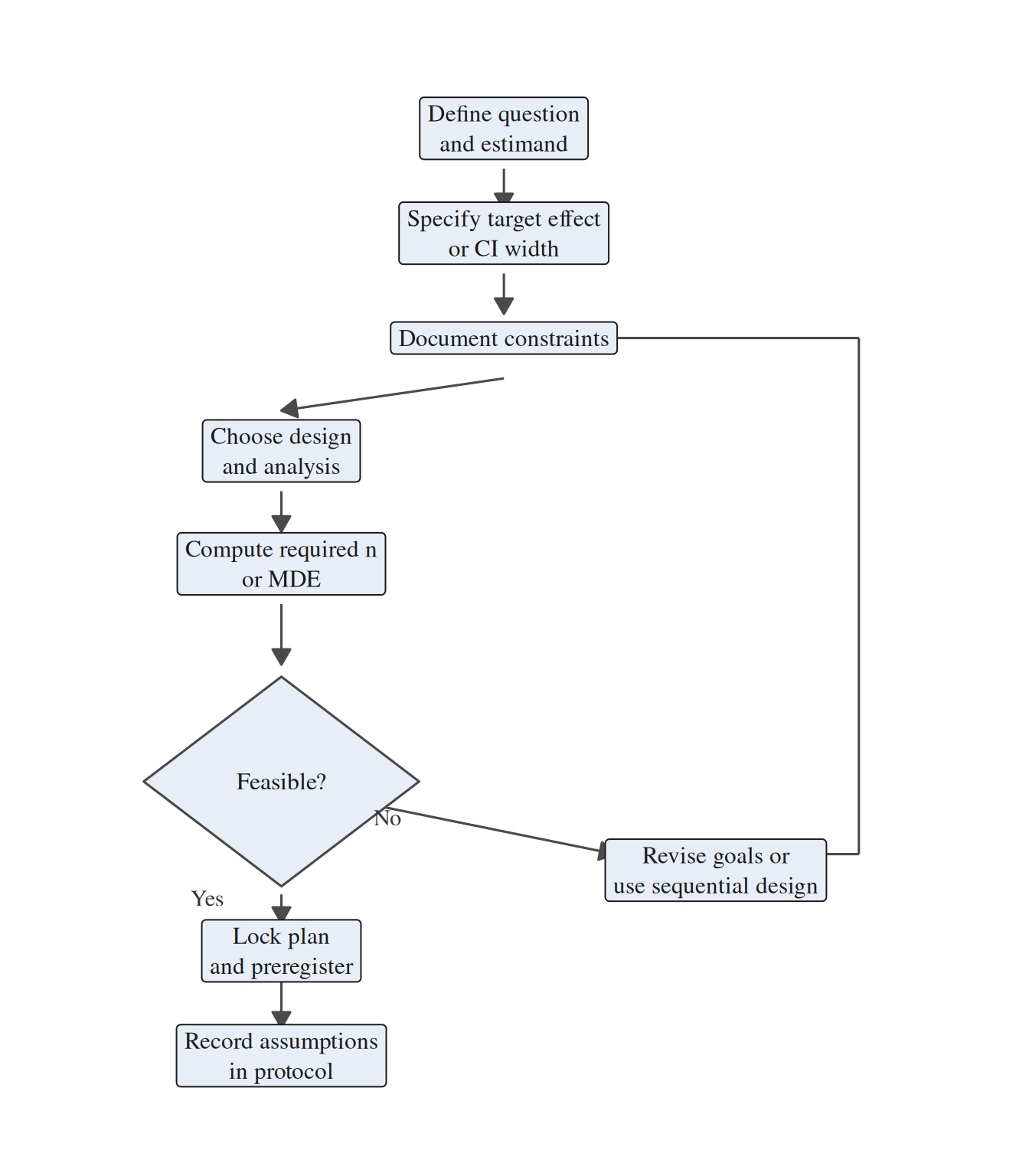
### Sample Size Planning Workflow
Integrating power analysis into a broader planning conversation prevents unrealistic promises and surfaces design trade-offs early. Use the following workflow whenever you scope a small-sample study:
1. **Clarify the question and estimand.** Identify the exact parameter the study needs to estimate, whether that is a difference in means, an odds ratio, a correlation, or some other target quantity.
2. **Specify tolerable uncertainty.** Define the minimum detectable effect or target confidence-interval width that would make the study actionable in substantive terms.
3. **Map constraints.** Document the recruitment limits, budget, timeline, and ethical restrictions that bound what the design can realistically support.
4. **Select design and analysis.** Choose the planned test or model, decide on one- versus two-sided inference, and note any covariates, matching, or repeated-measures structure.
5. **Compute required *n*.** Use analytical power formulas, simulation, or resampling as appropriate, and apply finite-population corrections if sampling without replacement from a known population.
6. **Assess feasibility.** Compare the required *n* with the constraints. If the target is infeasible, revise the design, narrow the claim, or shift the emphasis toward estimation or sequential decision-making.
7. **Document decisions.** Record the assumptions, software, code, and compromises so that readers can see exactly how the final sampling plan was chosen.
Figure 3.1 summarises the planning sequence and the point at which feasibility constraints feed back into design choices.
```{r}
#| label: qfig-ch3-sample-size-workflow
#| echo: false
#| fig-cap: "Figure 3.1: Sample size planning workflow for small studies."
#| alt: "Sample size planning workflow for small studies."
#| fig-width: 7
#| fig-height: 8
#| out-width: "82%"
library(grid)
box_nodes <- tibble(
id = c("q", "u", "c", "d", "n", "t", "r", "a"),
x = c(0, 0, 0, -2.1, -2.1, -2.1, -2.1, 2.0),
y = c(8.2, 6.9, 5.6, 4.2, 2.8, -2.0, -3.3, -1.0),
label = c(
"Define question\nand estimand",
"Specify target effect\nor CI width",
"Document constraints",
"Choose design\nand analysis",
"Compute required n\nor MDE",
"Lock plan\nand preregister",
"Record assumptions\nin protocol",
"Revise goals or\nuse sequential design"
)
)
decision_diamond <- tibble(
x = c(-2.1, -0.8, -2.1, -3.4),
y = c(1.4, 0.1, -1.2, 0.1)
)
line_segments <- tribble(
~x, ~y, ~xend, ~yend, ~arrowed,
0.0, 7.7, 0.0, 7.2, TRUE,
0.0, 6.4, 0.0, 5.9, TRUE,
0.0, 5.1, -2.1, 4.7, TRUE,
-2.1, 3.7, -2.1, 3.2, TRUE,
-2.1, 2.3, -2.1, 1.55, TRUE,
-2.1, -1.3, -2.1, -1.65, TRUE,
-2.1, -2.35, -2.1, -2.95, TRUE,
-1.2, -0.2, 1.05, -0.8, TRUE,
2.95, -0.8, 3.35, -0.8, FALSE,
3.35, -0.8, 3.35, 5.6, FALSE,
3.35, 5.6, 0.9, 5.6, TRUE
)
branch_labels <- tibble(
x = c(-2.8, -1.1),
y = c(-1.35, -0.35),
label = c("Yes", "No")
)
ggplot() +
geom_segment(
data = dplyr::filter(line_segments, !arrowed),
aes(x = x, y = y, xend = xend, yend = yend),
linewidth = 0.55,
colour = "#4A4A4A"
) +
geom_segment(
data = dplyr::filter(line_segments, arrowed),
aes(x = x, y = y, xend = xend, yend = yend),
linewidth = 0.55,
colour = "#4A4A4A",
arrow = arrow(length = unit(0.12, "inches"), type = "closed")
) +
geom_label(
data = box_nodes,
aes(x = x, y = y, label = label),
fill = "#E7EEF8",
colour = "#1A1A1A",
size = 4.1,
family = "serif",
label.size = 0.35,
label.padding = unit(0.28, "lines"),
label.r = unit(0.15, "lines"),
lineheight = 1.05
) +
geom_polygon(
data = decision_diamond,
aes(x = x, y = y),
fill = "#E7EEF8",
colour = "#4A4A4A",
linewidth = 0.55
) +
annotate(
"text",
x = -2.1,
y = 0.1,
label = "Feasible?",
family = "serif",
size = 4.2,
colour = "#1A1A1A"
) +
geom_text(
data = branch_labels,
aes(x = x, y = y, label = label),
family = "serif",
size = 4.0,
colour = "#333333"
) +
coord_cartesian(xlim = c(-4.0, 4.2), ylim = c(-3.9, 8.9), clip = "off") +
theme_void() +
theme(plot.margin = margin(10, 18, 10, 18))
```
Figure 3.1 makes the trade-off loop explicit: if the required sample size exceeds what is feasible, researchers can justify an exploratory framing, add interim analyses, or negotiate for additional resources before data collection begins.
### Justifying Small Sample Sizes
When sample sizes are constrained, the researcher's obligation is to be transparent rather than defensive. That means stating clearly both the target and accessible populations, describing the sampling method and the reasoning behind it, and reporting the planned and achieved sample sizes alongside power or precision estimates. If the study cannot detect effects of practical importance, that limitation should be acknowledged directly, and the findings should be framed as preliminary or exploratory when that description is accurate.
### Key Takeaways
Sampling in small studies is ultimately about aligning design ambitions with the population you can realistically reach. Probability sampling remains valuable when generalisation is the goal, but purposive, convenience, and quota approaches are often the feasible options in constrained settings and should be described honestly rather than overstated. Across all of these designs, transparent reporting of the sampling rationale, achieved sample, and detectable effect sizes is what allows readers to judge how much weight the findings can bear.
---
### Self-Assessment Quiz
Test your understanding of sampling strategies from Chapter 3.
```{r}
#| echo: false
#| results: asis
source(normalizePath(file.path(dirname(knitr::current_input(dir = TRUE)), "..", "R", "quiz_helpers.R"), mustWork = TRUE))
smallsamplelab_render_quiz(list(
list(
prompt = "A researcher uses a \"rule of thumb\" of n=30 per group for all studies. What is the primary problem with this approach?",
options = c("n=30 is always too small", "Sample size should depend on effect size, power, and research question—not arbitrary rules", "n=30 is always too large", "Rules of thumb are always correct"),
answer = 2L,
explanation = "Sample size should depend on effect size, power, and research question—not arbitrary rules. A small effect requires larger n; a large effect can be detected with smaller n. The chapter emphasizes: \"Rather than abandoning research in such contexts, we should adopt methods suited to smaller samples and report findings with appropriate caveats.\""
),
list(
prompt = "Stratified sampling is most useful when:",
options = c("The population is homogeneous", "You want to ensure representation of key subgroups that differ on the outcome", "Random selection is impossible", "Sample size exceeds 1,000"),
answer = 2L,
explanation = "Stratified sampling divides the population into strata and ensures each stratum is represented. This improves precision when strata differ on the outcome. The chapter states: \"Stratified sampling (dividing the population into strata and sampling proportionally or disproportionally from each) can improve precision by ensuring representation of key subgroups.\""
),
list(
prompt = "Power analysis reveals you need n=50 per group, but only n=20 is feasible. What should you do?",
options = c("Abandon the study", "Proceed, but report the study as exploratory/pilot and calculate minimum detectable effect (MDE)", "Proceed and claim the same statistical power", "Ignore power entirely"),
answer = 2L,
explanation = "Proceed, but report the study as exploratory/pilot and calculate minimum detectable effect (MDE). Transparency about power limitations is essential. The chapter recommends: \"If the achieved sample size is smaller than desired, report the minimum detectable effect (MDE).\""
),
list(
prompt = "Which sampling method allows probabilistic generalization to a target population?",
options = c("Convenience sampling", "Purposive sampling", "Simple random sampling", "Snowball sampling"),
answer = 3L,
explanation = "Simple random sampling (and other probability sampling methods) ensures every unit has a known, non-zero probability of selection, supporting generalization. The chapter states: \"Probability sampling...ensures that every unit has a known, non-zero probability of selection. This supports generalisation to the target population.\""
),
list(
prompt = "Quota sampling differs from stratified sampling in that:",
options = c("It uses random selection within strata", "It matches population proportions but does not use random selection", "It requires a sampling frame", "It is always more accurate"),
answer = 2L,
explanation = "Quota sampling matches population proportions but does not use random selection within strata. It \"mimics stratified sampling but without random selection within strata.\" This makes it non-probabilistic."
),
list(
prompt = "A study with n=15 per group has about 25% power to detect d=0.5. The researcher should report:",
options = c("\"The study was adequately powered\"", "\"The study was underpowered to detect medium effects; only very large effects (around d = 1.06) could be reliably detected\"", "\"Power is irrelevant with small samples\"", "\"Non-significant results prove no effect exists\""),
answer = 2L,
explanation = "With only about 25% power for d=0.5, the study is underpowered for medium effects. With n=15 per group, only very large effects, around d = 1.06 or larger, are close to the 80% power target. The chapter emphasizes transparent reporting: \"Researchers should conduct power analyses before data collection to understand what effects are detectable.\""
),
list(
prompt = "The finite population correction (FPC) is relevant when:",
options = c("Sampling with replacement from an infinite population", "Sampling without replacement from a small, known population (e.g., N=100)", "Sample size exceeds population size", "Using convenience sampling"),
answer = 2L,
explanation = "FPC adjusts required sample size when sampling without replacement from a small, finite population. The chapter explains: \"When sampling without replacement from a small, known population, the variance of estimates decreases...The finite population correction (FPC) adjusts the required sample size accordingly.\""
),
list(
prompt = "Sequential sampling allows researchers to:",
options = c("Collect all data simultaneously", "Stop early if interim results show sufficient precision or evidence", "Ignore power analysis", "Change hypotheses after seeing data"),
answer = 2L,
explanation = "Sequential sampling allows stopping early based on pre-specified decision rules if interim results show sufficient precision or evidence. The chapter describes: \"sequential designs allow researchers to review interim results and decide whether to continue sampling.\""
),
list(
prompt = "A convenience sample from one university is used to test a new teaching method. Which statement is TRUE?",
options = c("Results generalize to all universities", "Results are context-specific and require replication", "Convenience sampling is never acceptable", "Results are as valid as random sampling"),
answer = 2L,
explanation = "Convenience samples are context-specific and require replication. The chapter states: \"Findings from purposive or convenience samples should be interpreted cautiously and presented as preliminary or context-specific. Replication in independent samples strengthens confidence.\""
),
list(
prompt = "Minimum Detectable Effect (MDE) refers to:",
options = c("The smallest effect that exists in the population", "The smallest effect the study can detect with specified power (e.g., 80%)", "The p-value threshold", "The confidence interval width"),
answer = 2L,
explanation = "MDE is the smallest effect the study can detect with specified power (typically 80%) and alpha (typically 0.05). The chapter defines it: \"the minimum detectable effect (MDE): the smallest effect the study can detect with specified power.\""
)
))
```