Chapter 8: Handling Missing Data in Small Samples

Learning Objectives

By the end of this chapter, you will be able to distinguish MCAR, MAR, and MNAR mechanisms, describe missingness patterns clearly, judge when complete-case analysis or multiple imputation is defensible in a small sample, and report missing-data decisions with the transparency needed for readers to assess their consequences.

The Challenge of Missing Data in Small Samples

Missing data are common in applied research. Participants skip survey questions, drop out of longitudinal studies, or provide incomplete records. With large samples, modern methods (multiple imputation, full information maximum likelihood) can handle substantial missingness without excessive bias. With small samples, however, missing data pose severe problems. Even a few missing observations can substantially reduce effective sample size and statistical power.

Missing data methods rely on large-sample asymptotics and may be unstable or inappropriate when samples are very small (n < 30) or missingness is extensive (> 20%). In such cases, prevention (minimise missingness through careful design) and transparency (report missingness patterns and sensitivity analyses) are more important than sophisticated imputation.

Types of Missingness

The standard missingness framework distinguishes between three mechanisms (Rubin 1987; Buuren 2018). MCAR (Missing Completely At Random) means missingness is unrelated to any observed or unobserved variable, as when a survey page disappears because of a random software glitch. This condition is conceptually simple but rare in practice. MAR (Missing At Random) means missingness depends on observed variables but not on the missing values themselves once those observed variables are taken into account. For example, older participants may be more likely to skip a technology question, but conditional on age the missingness is otherwise random. MNAR (Missing Not At Random) is the hardest case because missingness depends on the unobserved values themselves, as when participants with severe depression are especially likely to drop out. That possibility cannot usually be resolved from the observed data alone and therefore requires sensitivity analysis or explicit modelling assumptions.

Describing Missingness Patterns

Before choosing a handling strategy, describe the pattern of missingness in plain terms. Report how many observations are missing on each variable, whether the missing values are concentrated in particular participants or particular variables, and whether incomplete cases differ from complete cases on observed characteristics that might make MAR more plausible than MCAR.

Example Dataset for Diagnostics

To demonstrate the handling strategies in this chapter, we simulate a small dataset with missing values on satisfaction and performance. Table 8.1 shows the first ten rows so the missing-data pattern is visible before the formal diagnostics begin.

Rendered Output

Table 8.1

Simulated study dataset with missing values (rows 1 to 10)

participant	age	satisfaction	performance
1	45	3	54
2	38	7	54
3	47	7	NA
4	53	5	68
5	42	3	72
6	36	5	51
7	43	3	84
8	37	5	49
9	34	4	66
10	46	4	61

Note. The full simulated dataset contains 25 participants; the excerpt is shown to illustrate the missing values before diagnosis.

Cell Code

Testing the MCAR Assumption

Little’s MCAR test evaluates whether missingness is consistent with the MCAR mechanism. The test compares observed means across missing-data patterns. A large p-value suggests MCAR is plausible, whereas a small p-value indicates that missingness likely depends on observed data (i.e., not MCAR). With small samples (n < 50), Little’s MCAR test has low power to detect meaningful departures from MCAR. A non-significant result does not confirm MCAR. Supplement it with visual inspection of missingness patterns, complete versus incomplete case comparisons, and substantive reasoning about why data might be missing (Graham 2009).

Rendered Output

Table 8.2

Little's MCAR test for the simulated study dataset

Statistic	df	p value	Missing patterns
13.309	6	0.038	3

Note. A larger p-value is more consistent with MCAR, but with small samples this test is only one piece of evidence and does not confirm MCAR. If the naniar package is unavailable, the table records the number of observed missingness patterns and the formal test should be run before final reporting.

Figure 8.1: Percentage of missing values per variable.

Cell Code

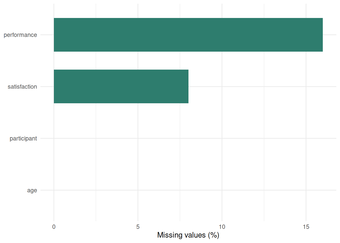
Little’s MCAR test assesses whether missing data patterns are completely random. Table 8.2 reports the test statistics, while Figure 8.1 shows the percentage of missing values for each variable. However, with small samples (n < 50), the test has low power and should be treated as one clue rather than a verdict. In practice, it should be supplemented with visual inspection of missingness patterns, comparisons between complete and incomplete cases, and domain knowledge about why participants might have skipped particular items or visits.

Observation-Level Missingness Pattern

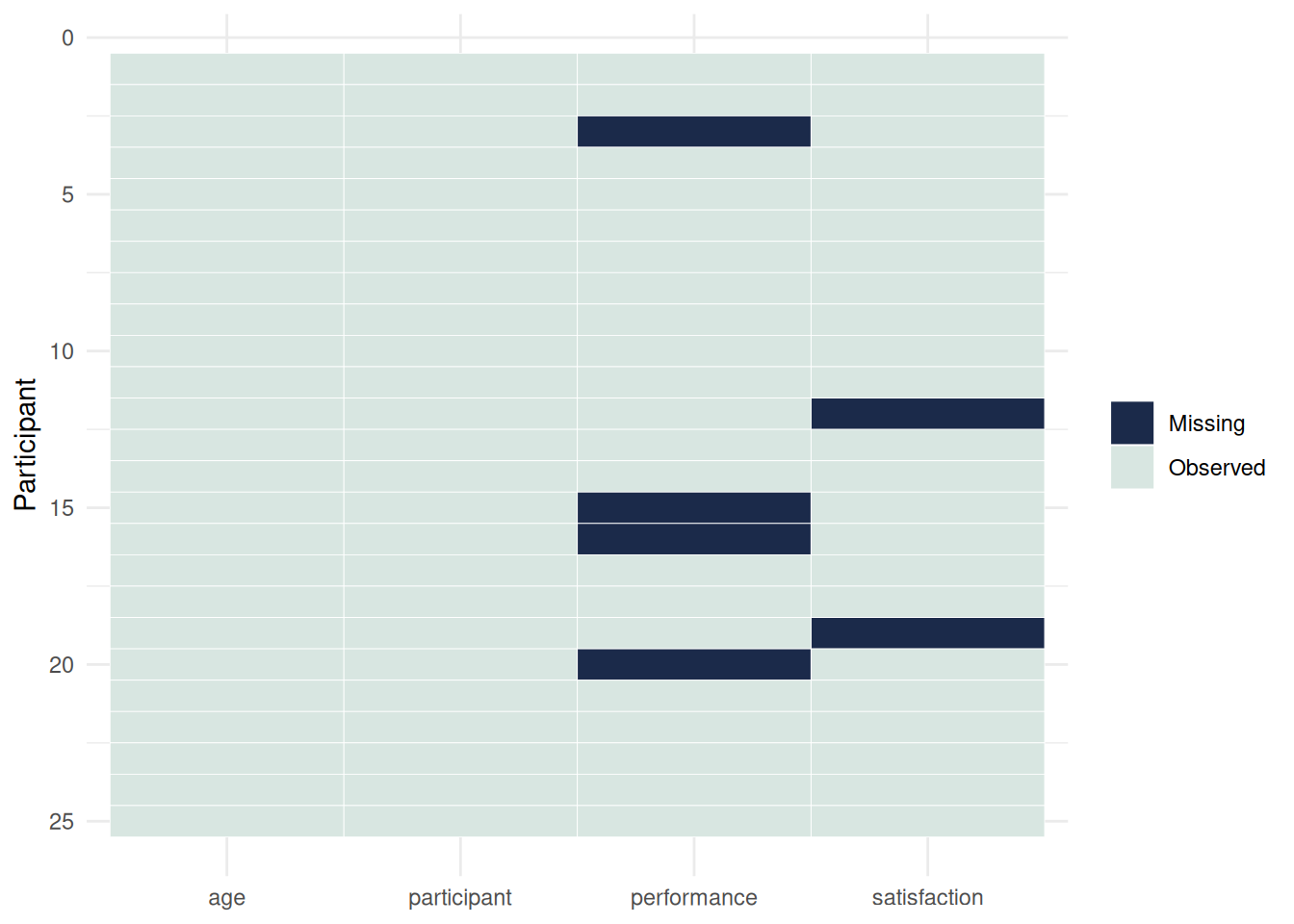
Figure 8.2 complements Figure 8.1 by showing whether missing values cluster within particular cases rather than only within particular variables.

Rendered Output

Figure 8.2: Observation-level missingness pattern.

Cell Code

Example: Summarising Missing Data

We continue working with the simulated dataset (study_data) created above. Tables 8.3 to 8.5 summarise how much data are missing and whether the incomplete cases differ from the complete cases on age.

Rendered Output

Table 8.3

Number of missing values by variable

Variable	Missing
participant	0
age	0
satisfaction	2
performance	4

Table 8.4

Proportion of missing values by variable

Variable	Proportion missing
participant	0.00
age	0.00
satisfaction	0.08
performance	0.16

Table 8.5

Age comparison for complete and incomplete cases

Group	Mean age	n
Incomplete	39.8	6
Complete	41.9	19

Cell Code

Interpretation: Tables 8.3 and 8.4 show that performance has the heaviest missingness burden, at about 20% of the sample. Table 8.5 then shows that the incomplete cases are younger on average than the complete cases, which makes MCAR less automatic and suggests that MAR or MNAR should remain plausible possibilities. With 20% missingness and n = 25, only 20 cases remain in a complete-case analysis, so power is reduced sharply.

Complete-Case (Listwise Deletion) Analysis

The simplest approach is to analyse only cases with complete data on all variables of interest. This is valid if missingness is MCAR and the reduction in sample size is tolerable. However, it can introduce bias if missingness is MAR or MNAR, and it wastes information. Complete-case analysis is most defensible when missingness is minimal, MCAR is at least plausible, or the sample is so small that a more elaborate imputation model would be less credible than a transparent analysis of the observed cases.

WarningCommon Misconception: “Listwise Deletion Is Always Safe if Missingness Is Random”

Myth: “If I check for MCAR and the test is non-significant, listwise deletion is unbiased.”

Reality: Even when missingness is truly MCAR, listwise deletion loses power and can introduce bias if you have multiple variables with independent missing patterns.

Demonstration:

set.seed(2025)

# Generate complete data: n=50, correlation between x and y = 0.6
n <- 50
x <- rnorm(n, 50, 10)
y <- 0.6 * x + rnorm(n, 0, 8)

# True correlation (no missing data)
true_cor <- cor(x, y)

# Introduce MCAR missingness (20% on x, 20% on y, independently)
x_missing <- x
y_missing <- y
x_missing[sample(1:n, 10)] <- NA  # 20% missing
y_missing[sample(1:n, 10)] <- NA  # 20% missing

# Listwise deletion: only cases with both x and y
complete_cases <- complete.cases(x_missing, y_missing)

# Correlation with listwise deletion
listwise_cor <- cor(x_missing[complete_cases], y_missing[complete_cases])

listwise_demo <- tibble(
  Metric = c(
    "True correlation (complete data)",
    "Complete cases retained",
    "Correlation after listwise deletion",
    "Cases lost",
    "Standard error inflation"
  ),
  Value = c(
    formatC(true_cor, format = "f", digits = 3),
    sprintf("%d / %d (%.1f%%)", sum(complete_cases), n, 100 * mean(complete_cases)),
    formatC(listwise_cor, format = "f", digits = 3),
    sprintf("%d (%.1f%%)", n - sum(complete_cases), 100 * (1 - mean(complete_cases))),
    sprintf("%.2f×", sqrt(1 / sum(complete_cases)) / sqrt(1 / n))
  )
)

smallsamplelab_apa_table(
  "8.6",
  "Consequences of listwise deletion under independent MCAR missingness",
  listwise_demo,
  note = "With 20% missing on x and 20% missing on y, independent MCAR retention is (1 - p1) x (1 - p2) = 0.8 x 0.8 = 0.64, so only about 64% of cases remain once both variables are required.",
  align = c("l", "l")
)

Table 8.6

Consequences of listwise deletion under independent MCAR missingness

Metric	Value
True correlation (complete data)	0.549
Complete cases retained	33 / 50 (66.0%)
Correlation after listwise deletion	0.548
Cases lost	17 (34.0%)
Standard error inflation	1.23×

Note. With 20% missing on x and 20% missing on y, independent MCAR retention is (1 - p1) x (1 - p2) = 0.8 x 0.8 = 0.64, so only about 64% of cases remain once both variables are required.

Why this matters:

1. Power loss: With 20% missing on x and 20% on y independently, the retention rate is (1 - p_x) x (1 - p_y) = 0.8 x 0.8 = 0.64, so about 36% of cases are lost.
2. Multiple variables compound: With five variables each 15% missing, the retention rate is 0.85^5 = 0.44, so less than half the sample remains.
3. Bias can still occur: If missingness is MAR rather than MCAR, listwise deletion can bias estimates as well as reduce precision.

Lesson:

• MCAR does NOT mean listwise deletion is optimal—it can still waste information.
• Consider multiple imputation when missingness exceeds about 10%, the sample is large enough for the imputation model, and MAR is plausible.
• With small samples (n < 50), losing even 20% of cases can sharply reduce power.

When listwise deletion is actually safe:

• Missingness < 5% on any variable
• n is large enough that losing cases doesn’t hurt power
• You’ve verified MCAR (not just MAR) AND documented the power loss

Mean Imputation (Not Recommended)

Mean imputation replaces missing values with the variable mean. This approach artificially reduces variance and distorts correlations. It is generally not recommended, especially with small samples where each imputed value has disproportionate impact. At most, it might be tolerated for trivial descriptive summaries in a much larger dataset, but it should not be treated as an inferential solution.

Last Observation Carried Forward (LOCF)

In longitudinal studies, LOCF replaces missing follow-up values with the last observed value for that individual. This assumes no change after the last observation, which is often unrealistic. LOCF can therefore bias estimates and is not generally recommended. It is only marginally defensible when the assumption of no meaningful change is substantively plausible and no better alternative is available.

Multiple Imputation (Caution with Small Samples)

Multiple imputation (MI) generates several plausible imputed datasets, analyses each separately, and pools results to account for imputation uncertainty. MI is a strong default for handling missing data in adequately sized samples when MAR is plausible (Rubin 1987; White, Royston, and Wood 2011; Buuren 2018). If MNAR is suspected, MI alone does not solve the problem. The practical response is sensitivity analysis that varies the assumed departure from MAR (Sterne et al. 2009). MI requires sufficient data to estimate imputation models reliably. With very small samples (n < 30) or extensive missingness (> 20%), imputation models may be under-identified and can yield unstable or implausible imputations. If MI is attempted in that setting, use predictive mean matching (method = "pmm"), limit the number of predictors in the imputation model, check convergence diagnostics carefully, and report complete-case results as a sensitivity check.

Example: Multiple Imputation with mice (Caution)

We apply MI to the dataset with missing satisfaction and performance values. Given the small sample (n = 25) and 20% missingness, interpret results cautiously. Table 8.7 reports the pooled regression results rather than printing the raw imputation object.

Rendered Output

Table 8.7

Pooled regression results from the illustrative multiple-imputation analysis

Term	Estimate	Std. error	Statistic	p value
(Intercept)	55.443	11.716	4.73	0.000
age	0.566	0.186	3.05	0.007
satisfaction	-3.379	1.608	-2.10	0.054

Note. Five predictive-mean-matching imputations were pooled using Rubin's rules. With only 25 cases and 20% missingness, these estimates should be treated as provisional.

Cell Code

Interpretation: MI generates plausible values for missing data based on observed relationships. The pooled results combine estimates across imputations, with standard errors adjusted for imputation uncertainty. However, with n = 25 and 20% missingness, the imputation model is estimated from limited data, and results may be unstable. Before reporting the pooled estimates, inspect the standard mice trace plots with plot(imp) and increase maxit or simplify the imputation model if the chains drift rather than forming a stable fuzzy pattern. Compare MI results to complete-case analysis. If they differ substantially, report both and acknowledge uncertainty. Record the random seed, imputation method, number of imputations, and package versions whenever stochastic imputation code is adapted.

Checking Convergence of Multiple Imputation

When using mice, always check whether the imputation algorithm has converged. Poor convergence means the imputed values may not be stable, especially with small samples or complex missing data patterns. This chapter keeps the emphasis on handling decisions rather than diagnostic graphics, so the detailed trace-plot and strip-plot workflow is taken up in Chapter 9: For the present chapter, the practical takeaway is that any MI analysis should be accompanied by those diagnostics before it is reported as credible.

Sensitivity Analyses

When missingness is substantial or MNAR is suspected, conduct sensitivity analyses rather than presenting a single imputed answer as definitive. Compare complete-case results with imputed results, vary the assumptions about the missing-data mechanism where possible, and report how much the substantive conclusions change across those scenarios.

Preventing Missing Data

The best approach to missing data is still prevention. Clear instruments, low respondent burden, follow-up for missed appointments or skipped questions, pilot testing of confusing procedures, and good rapport with participants all reduce the need for heroic statistical repair later.

Key Takeaways

Missing-data work in small samples begins with description, not imputation. Researchers need to know how much is missing, where it is missing, and which missingness mechanisms are plausible before choosing a handling strategy. Complete-case analysis can be acceptable in narrowly defined situations but often wastes too much information, while multiple imputation is only as credible as the sample size, missingness level, and modelling assumptions allow. That is why prevention, diagnostics, and sensitivity analysis matter as much as the final pooled estimate.

Self-Assessment Quiz

Test your understanding of missing-data decisions in Chapter 8.

Question 1. What is the key distinction between MCAR and MAR?

MCAR means no data are missing; MAR means some data are missingMCAR means missingness is unrelated to observed or unobserved data, whereas MAR allows missingness to depend on observed variablesMCAR applies only to experiments; MAR applies only to surveysThere is no practical difference between them

Explanation.

The chapter defines MCAR as missingness unrelated to any variables and MAR as missingness related to observed variables but not the missing values themselves. This distinction matters because most modern missing-data methods assume MAR, not MCAR.

Question 2. Why can listwise deletion still be a poor choice even when MCAR is plausible?

It always creates impossible valuesIt can throw away many cases and sharply reduce power, especially when missingness occurs on multiple variablesIt is only allowed in Bayesian analysisIt automatically changes MAR data into MNAR data

Explanation.

The chapter’s misconception box shows that independent missingness across variables compounds quickly. Even under MCAR, listwise deletion can waste a large fraction of a small dataset and make estimates much less precise.

Question 3. Why is mean imputation generally not recommended?

It is too computationally expensiveIt artificially reduces variance and distorts associations between variablesIt requires a larger sample than multiple imputationIt only works for binary outcomes

Explanation.

Mean imputation replaces uncertainty with a constant value. The chapter warns that this shrinks variability and biases correlations, which is especially damaging when each observation matters.

Question 4. When is multiple imputation most defensible in this chapter’s guidance?

When n is moderate, missingness is not too extensive, and MAR is plausibleWhenever a dataset contains any missing value at allOnly when data are MNAROnly when the outcome is binary

Explanation.

The chapter describes multiple imputation as most appropriate when the sample is not extremely small, missingness is moderate, and the MAR assumption is plausible. It explicitly cautions that MI can be unstable with n < 30 or heavy missingness.

Question 5. Why is last observation carried forward (LOCF) usually a weak solution to missing follow-up data?

Because it assumes no meaningful change after the last observed valueBecause it can only be used with binary outcomesBecause it always increases statistical powerBecause it requires Bayesian software

Explanation.

The chapter warns that LOCF assumes the participant would have stayed unchanged after the last observed value. That assumption is often unrealistic, so LOCF can bias treatment effects or longitudinal trends.

Question 6. What does Little’s MCAR test evaluate?

Whether missingness is consistent with a completely-random mechanismWhether multiple imputation has convergedWhether the outcome is normally distributedWhether LOCF is acceptable

Explanation.

Little’s MCAR test compares observed means across missing-data patterns to assess whether the data are consistent with MCAR. The chapter also stresses that, with small samples, this test is only one clue rather than a final verdict.

Question 7. Why are sensitivity analyses important for missing-data work?

They prove which missingness mechanism is correctThey show whether conclusions depend heavily on the assumptions used to handle missing dataThey eliminate the need to describe missingness patternsThey allow you to ignore complete-case results

Explanation.

Because the missingness mechanism is often uncertain, the chapter recommends comparing results under different reasonable assumptions. If results change materially, that uncertainty should be reported rather than hidden.

Question 8. What is the best overall strategy for dealing with missing data in small-sample studies?

Prevent as much missingness as possible through study design and follow-upDefault to mean imputation because it is simpleAlways drop incomplete cases regardless of contextAssume MCAR unless the sample is very large

Explanation.

The chapter ends by stressing prevention: clear instruments, reduced burden, follow-up procedures, and pilot testing. No statistical fix can fully recover information that was never observed.

Ayre, Colin, and Andrew J. Scally. 2014. ‘Critical Values for Lawshe’s Content Validity Ratio: Revisiting the Original Methods of Calculation’. Measurement and Evaluation in Counseling and Development 47 (1): 79–86. https://doi.org/10.1177/0748175613513808.

Briggs, Steven R., and Jonathan M. Cheek. 1986. ‘The Role of Factor Analysis in the Development and Evaluation of Personality Scales’. Journal of Personality 54 (1): 106–48.

Buuren, Stef van. 2018. Flexible Imputation of Missing Data. 2nd ed. Boca Raton, FL: Chapman; Hall/CRC.

Cameron, A. Colin, and Pravin K. Trivedi. 2013. Regression Analysis of Count Data. 2nd ed. Cambridge: Cambridge University Press. https://doi.org/10.1017/CBO9781139013567.

Chen, Henian, Patricia Cohen, and Sophie Chen. 2010. ‘How Big Is a Big Odds Ratio? Interpreting the Magnitudes of Odds Ratios in Epidemiological Studies’. Communications in Statistics - Simulation and Computation 39 (4): 860–64. https://doi.org/10.1080/03610911003650383.

Cicchetti, Domenic V. 1994. ‘Guidelines, Criteria, and Rules of Thumb for Evaluating Normed and Standardized Assessment Instruments in Psychology’. Psychological Assessment 6 (4): 284–90. https://doi.org/10.1037/1040-3590.6.4.284.

Clark, Lee Anna, and David Watson. 1995. ‘Constructing Validity: Basic Issues in Objective Scale Development’. Psychological Assessment 7 (3): 309–19.

Cohen, Jacob. 1988. Statistical Power Analysis for the Behavioral Sciences. 2nd ed. Hillsdale, NJ: Lawrence Erlbaum Associates.

Conover, W. J. 1999. Practical Nonparametric Statistics. 3rd ed. New York: John Wiley & Sons.

Costello, Anna B., and Jason Osborne. 2005. ‘Best Practices in Exploratory Factor Analysis: Four Recommendations for Getting the Most from Your Analysis’. Practical Assessment, Research, and Evaluation 10 (1): 1–9. https://doi.org/10.7275/jyj1-4868.

Davison, A. C., and D. V. Hinkley. 1997. Bootstrap Methods and Their Application. Cambridge Series in Statistical and Probabilistic Mathematics. Cambridge: Cambridge University Press.

DeVellis, Robert F., and Carolyn T. Thorpe. 2021. Scale Development: Theory and Applications. 5th ed. Thousand Oaks, CA: SAGE Publications.

Dienes, Zoltan. 2014. ‘Using Bayes to Get the Most Out of Non-Significant Results’. Frontiers in Psychology 5: 781. https://doi.org/10.3389/fpsyg.2014.00781.

Efron, Bradley, and Robert J. Tibshirani. 1993. An Introduction to the Bootstrap. New York, NY: Chapman; Hall/CRC.

Elm, Erik von, Douglas G. Altman, Matthias Egger, Stuart J. Pocock, Peter C. Gøtzsche, and Jan P. Vandenbroucke. 2007. ‘The Strengthening the Reporting of Observational Studies in Epidemiology (STROBE) Statement: Guidelines for Reporting Observational Studies’. PLoS Medicine 4 (10): e296. https://doi.org/10.1371/journal.pmed.0040296.

Fay, Michael P. 2010. ‘Confidence Intervals That Match Fisher’s Exact or Blaker’s Exact Tests’. Biostatistics 11 (2): 373–74. https://doi.org/10.1093/biostatistics/kxp050.

Firth, David. 1993. ‘Bias Reduction of Maximum Likelihood Estimates’. Biometrika 80 (1): 27–38. https://doi.org/10.1093/biomet/80.1.27.

Gelman, Andrew, Daniel Simpson, and Michael Betancourt. 2017. ‘The Prior Can Often Only Be Understood in the Context of the Likelihood’. Entropy 19 (10): 555. https://doi.org/10.3390/e19100555.

Good, Phillip I. 2005. Permutation, Parametric, and Bootstrap Tests of Hypotheses. 3rd ed. New York: Springer.

Graham, John W. 2009. ‘Missing Data Analysis: Making It Work in the Real World’. Annual Review of Psychology 60: 549–76. https://doi.org/10.1146/annurev.psych.58.110405.085530.

Hair, Joseph F., G. Tomas M. Hult, Christian M. Ringle, and Marko Sarstedt. 2017. A Primer on Partial Least Squares Structural Equation Modeling (PLS-SEM). 2nd ed. Thousand Oaks, CA: SAGE Publications.

Harrell, Frank E. 2015. Regression Modeling Strategies: With Applications to Linear Models, Logistic and Ordinal Regression, and Survival Analysis. 2nd ed. Springer Series in Statistics. New York: Springer. https://doi.org/10.1007/978-3-319-19425-7.

Heinze, Georg, and Michael Schemper. 2002. ‘A Solution to the Problem of Separation in Logistic Regression’. Statistics in Medicine 21 (16): 2409–19. https://doi.org/10.1002/sim.1047.

Hodges, Jr., J. L., and E. L. Lehmann. 1963. ‘Estimates of Location Based on Rank Tests’. The Annals of Mathematical Statistics 34 (2): 598–611. https://doi.org/10.1214/aoms/1177704172.

Hoenig, John M., and Dennis M. Heisey. 2001. ‘The Abuse of Power: The Pervasive Fallacy of Power Calculations for Data Analysis’. The American Statistician 55 (1): 19–24.

Hosmer, David W., Stanley Lemeshow, and Rodney X. Sturdivant. 2013. Applied Logistic Regression. 3rd ed. Wiley Series in Probability and Statistics. Hoboken, NJ: John Wiley & Sons. https://doi.org/10.1002/9781118548387.

Hu, Li-tze, and Peter M. Bentler. 1999. ‘Cutoff Criteria for Fit Indexes in Covariance Structure Analysis: Conventional Criteria Versus New Alternatives’. Structural Equation Modeling 6 (1): 1–55. https://doi.org/10.1080/10705519909540118.

Huberty, Carl J., and Stephen Olejnik. 2006. Applied MANOVA and Discriminant Analysis. 2nd ed. Hoboken, NJ: Wiley. https://doi.org/10.1002/047178947X.

Hwang, Ching-Lai, and Kwangsun Yoon. 1981. Multiple Attribute Decision Making: Methods and Applications. Berlin: Springer. https://doi.org/10.1007/978-3-642-48318-9.

Hyndman, Rob J., and George Athanasopoulos. 2021. Forecasting: Principles and Practice. 3rd ed. Melbourne, Australia: OTexts. https://otexts.com/fpp3/.

Koo, Terry K., and Mae Y. Li. 2016. ‘A Guideline of Selecting and Reporting Intraclass Correlation Coefficients for Reliability Research’. Journal of Chiropractic Medicine 15 (2): 155–63. https://doi.org/10.1016/j.jcm.2016.02.012.

Kraft, Matthew A. 2020. ‘Interpreting Effect Sizes of Education Interventions’. Educational Researcher 49 (4): 241–53. https://doi.org/10.3102/0013189X20912798.

Lakens, Daniël. 2013. ‘Calculating and Reporting Effect Sizes to Facilitate Cumulative Science: A Practical Primer for t-Tests and ANOVAs’. Frontiers in Psychology 4: 863. https://doi.org/10.3389/fpsyg.2013.00863.

Lakens, Daniël, Anne M. Scheel, and Peder M. Isager. 2018. ‘Equivalence Testing for Psychological Research: A Tutorial’. Advances in Methods and Practices in Psychological Science 1 (2): 259–69. https://doi.org/10.1177/2515245918770963.

Lawshe, Charles H. 1975. ‘A Quantitative Approach to Content Validity’. Personnel Psychology 28 (4): 563–75. https://doi.org/10.1111/j.1744-6570.1975.tb01393.x.

Lipsey, Mark W., and David B. Wilson. 1993. ‘The Efficacy of Psychological, Educational, and Behavioural Treatment: Confirmation from Meta-Analysis’. American Psychologist 48 (12): 1181–1209. https://doi.org/10.1037/0003-066X.48.12.1181.

Little, Roderick J. A. 1988. ‘A Test of Missing Completely at Random for Multivariate Data with Missing Values’. Journal of the American Statistical Association 83 (404): 1198–1202. https://doi.org/10.1080/01621459.1988.10478722.

MacKinnon, David P., Jennifer L. Krull, and Chondra M. Lockwood. 2000. ‘Equivalence of the Mediation, Confounding and Suppression Effect’. Prevention Science 1 (4): 173–81.

Mair, Patrick, and Rand R. Wilcox. 2020. ‘Robust Statistical Methods in r Using the WRS2 Package’. Behavior Research Methods 52 (2): 464–88. https://doi.org/10.3758/s13428-019-01246-w.

Mann, Henry B., and Donald R. Whitney. 1947. ‘On a Test of Whether One of Two Random Variables Is Stochastically Larger Than the Other’. The Annals of Mathematical Statistics 18 (1): 50–60. https://doi.org/10.1214/aoms/1177730491.

McDonald, Roderick P. 1999. Test Theory: A Unified Treatment. Mahwah, NJ: Lawrence Erlbaum Associates.

Morey, Richard D., and Jeffrey N. Rouder. 2011. ‘Bayes Factor Approaches for Testing Interval Null Hypotheses’. Psychological Methods 16 (4): 406–19. https://doi.org/10.1037/a0024377.

Nielsen, Jakob. 1993. Usability Engineering. San Francisco, CA: Morgan Kaufmann.

Olsson, Ulf. 1979. ‘Maximum Likelihood Estimation of the Polychoric Correlation Coefficient’. Psychometrika 44 (4): 443–60.

Opricovic, Serafim, and Gwo-Hshiung Tzeng. 2004. ‘Compromise Solution by MCDM Methods: A Comparative Analysis of VIKOR and TOPSIS’. European Journal of Operational Research 156 (2): 445–55. https://doi.org/10.1016/S0377-2217(03)00020-1.

Page, Matthew J., Joanne E. McKenzie, Patrick M. Bossuyt, Isabelle Boutron, Tammy C. Hoffmann, Cynthia D. Mulrow, Larissa Shamseer, et al. 2021. ‘The PRISMA 2020 Statement: An Updated Guideline for Reporting Systematic Reviews’. BMJ 372: n71. https://doi.org/10.1136/bmj.n71.

R Core Team. 2026. R: A Language and Environment for Statistical Computing. Vienna, Austria: R Foundation for Statistical Computing. https://www.R-project.org/.

Rubin, Donald B. 1987. Multiple Imputation for Nonresponse in Surveys. New York, NY: Wiley.

Saaty, Thomas L. 1980. The Analytic Hierarchy Process. New York, NY: McGraw-Hill.

Schulz, Kenneth F., Douglas G. Altman, and David Moher. 2010. ‘CONSORT 2010 Statement: Updated Guidelines for Reporting Parallel Group Randomised Trials’. BMJ 340: c332. https://doi.org/10.1136/bmj.c332.

Shan, Guogen. 2018. Exact Statistical Inference for Categorical Data. London: Academic Press.

Sterne, Jonathan A. C., Ian R. White, John B. Carlin, Michael Spratt, Patrick Royston, Michael G. Kenward, Angela M. Wood, and James R. Carpenter. 2009. ‘Multiple Imputation for Missing Data in Epidemiological and Clinical Research: Potential and Pitfalls’. BMJ 338: b2393. https://doi.org/10.1136/bmj.b2393.

Teare, M. Dawn, Munyaradzi Dimairo, Neil Shephard, Amanda Hayman, Amy Whitehead, and Stephen J. Walters. 2014. ‘Sample Size Requirements to Estimate Key Design Parameters from External Pilot Randomised Controlled Trials: A Simulation Study’. Trials 15: 264. https://doi.org/10.1186/1745-6215-15-264.

Tomczak, Maciej, and Ewa Tomczak. 2014. ‘The Need to Report Effect Size Estimates Revisited: An Overview of Some Recommended Measures of Effect Size’. Trends in Sport Sciences 21 (1): 19–25.

Trizano-Hermosilla, Italo, and Jose M. Alvarado. 2016. ‘Best Alternatives to Cronbach’s Alpha Reliability in Realistic Conditions: Congeneric and Asymmetrical Measurements’. Frontiers in Psychology 7: 769. https://doi.org/10.3389/fpsyg.2016.00769.

Van de Schoot, Rens, and Milica Miočević. 2020. Small Sample Size Solutions: A Guide for Applied Researchers and Practitioners. London: Routledge.

Vehtari, Aki, Andrew Gelman, and Jonah Gabry. 2017. ‘Practical Bayesian Model Evaluation Using Leave-One-Out Cross-Validation and WAIC’. Statistics and Computing 27 (5): 1413–32. https://doi.org/10.1007/s11222-016-9696-4.

Wagenmakers, Eric-Jan, Jonathon Love, Maarten Marsman, Tahira Jamil, Alexander Ly, Josine Verhagen, Ravi Selker, et al. 2018. ‘Bayesian Inference for Psychology. Part II: Example Applications with JASP’. Psychonomic Bulletin & Review 25 (1): 58–76. https://doi.org/10.3758/s13423-017-1323-7.

White, Ian R., Patrick Royston, and Angela M. Wood. 2011. ‘Multiple Imputation Using Chained Equations: Issues and Guidance for Practice’. Statistics in Medicine 30 (4): 377–99. https://doi.org/10.1002/sim.4067.