Chapter 13: Penalised and Bayesian Regression for Small Samples

Learning Objectives

By the end of this chapter, you will be able to explain why ordinary maximum likelihood can fail with sparse regression data, recognise separation in logistic regression, use penalised estimates to stabilise small-sample models, describe how weakly informative Bayesian priors regularise estimates, and report sensitivity checks without presenting regularisation as a substitute for information.

The Problem of Sparse Data in Regression

Classical maximum likelihood estimation can become unstable when sample sizes are small, events are rare, or predictors nearly separate outcome groups. In logistic regression, separation occurs when a predictor or predictor combination nearly or perfectly predicts the binary outcome. The fitted probabilities then approach 0 or 1, coefficient estimates become very large, and Wald standard errors stop being useful. A practical diagnostic is to inspect simple predictor-by-outcome tables for zero cells and to check whether the logistic model warns that fitted probabilities are numerically 0 or 1.

Penalised regression and Bayesian regression respond to the same problem in different language. Penalised regression adds a constraint to the likelihood so that extreme coefficients are pulled back toward more stable values. Bayesian regression combines the likelihood with prior distributions. Weakly informative priors serve as regularisation when the data alone are too thin to support precise estimates. Neither approach creates information that is not in the data. Both make the modelling assumptions more explicit.

Choosing Among Regularisation Strategies

Regularisation covers a family of strategies, and the appropriate choice depends on the outcome, the modelling goal, and the specific source of instability.

Problem in the small dataset	Better starting point	Why
Sparse binary outcome or separation warnings in logistic regression	Firth logistic regression	Produces finite bias-reduced estimates when ordinary maximum likelihood breaks down
Continuous outcome with correlated predictors	Ridge regression	Shrinks all slopes and reduces instability from collinearity without selecting a single “winner”
Continuous outcome with many candidate predictors and a screening goal	LASSO	Can set weak or unstable coefficients to zero, but selection should be treated as exploratory
Strong prior knowledge or a need to express assumptions directly	Bayesian regression with weakly informative priors	Regularises estimates through explicit prior distributions and requires convergence checks
Main goal is explanation of one pre-specified effect	Simpler pre-specified model plus sensitivity analysis	Penalised selection can obscure the estimand if the target effect was already known
Main goal is prediction	Penalised model with transparent tuning and validation	Prediction requires checking out-of-sample behaviour, not only coefficient significance

For small samples, the safest workflow is to fit the simplest scientifically meaningful model first, then use regularised estimates as sensitivity checks or as explicitly labelled prediction tools. If regularisation changes the substantive conclusion, report that instability rather than hiding it behind a single preferred model.

Firth-Penalised Logistic Regression

Firth’s method reduces small-sample bias in likelihood estimation and is especially useful for sparse binary outcomes or separation (Firth 1993; Heinze and Schemper 2002). Table 13.1 shows the structure of a small project-success example. Most low-planning projects fail and most high-planning projects succeed, which creates a separation risk.

Table 13.1

Sparse project-success data used for the logistic-regression example

Planning band	No success	Success	Success rate
Planning score 1-5	11	1	8%
Planning score 6-9	0	8	100%

Note. The outcome is nearly separated by planning score. This is the setting where ordinary logistic regression can produce unstable estimates.

The ordinary logistic model fits in R, but the fitted probabilities are close to 0 or 1. That is a warning sign even if the software returns coefficients. Table 13.2 compares ordinary maximum-likelihood estimates with Firth-penalised estimates when the logistf package is available.

Table 13.2

Standard and Firth-penalised logistic-regression estimates

Method	Term	Estimate	Std. error	p-value
Standard ML	Planning score	43.85	42168.42	0.999
Standard ML	Prior experience	44.72	57464.52	0.999
Firth	Planning score	1.02	0.80	0.218
Firth	Prior experience	1.66	1.54	0.328

Note. The standard-model standard errors are Wald estimates from glm(); under separation they can become extremely large or effectively unbounded, especially when R warns that fitted probabilities are numerically 0 or 1. In this example, fitted probabilities close to 0 or 1 occurred: yes. Use logistf or another penalised method immediately when that warning appears. Firth's method adds a penalty proportional to the log determinant of the Fisher information matrix, reducing small-sample bias and preventing infinite estimates under separation. Coefficients remain on the log-odds scale and can be exponentiated for odds-ratio interpretation.

Interpretation should focus on direction, uncertainty, and model fragility. A finite Firth coefficient is a more stable estimate under a penalised likelihood, not confirmation that the effect size is precisely known. In small samples, report the event counts, variables in the model, penalisation method, confidence intervals, and whether ordinary logistic regression showed separation warnings.

Ridge Regression as Shrinkage

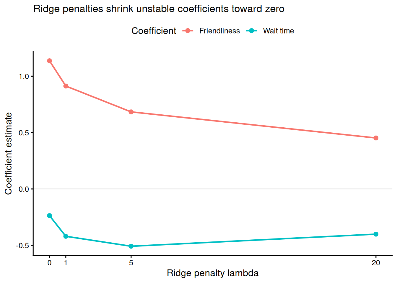
Ridge regression shrinks regression coefficients toward zero by adding a penalty proportional to the squared coefficient size. It is useful when predictors are correlated, sample size is modest, or the goal is prediction rather than unpenalised coefficient interpretation (Harrell 2015). Table 13.3 and Figure 13.1 show the same small customer-satisfaction regression under increasing ridge penalties.

Table 13.3

Ridge coefficient estimates under increasing penalty strength

Lambda	Intercept	Wait time	Friendliness
0	5.94	-0.24	1.14
1	5.94	-0.42	0.91
5	5.94	-0.51	0.68
20	5.94	-0.40	0.45

Note. Predictors were standardised to mean = 0 and SD = 1 before fitting because the L2 penalty is scale-dependent. Lambda = 0 is the ordinary least-squares solution. Coefficients apply to standardised predictors unless back-transformed.

Figure 13.1: Ridge coefficient paths for the customer-satisfaction example.

As lambda increases, the slope estimates move toward zero. That shrinkage can reduce overfitting and improve prediction, but it also changes the estimand: the coefficients are penalised estimates, not ordinary least-squares coefficients. Report the penalty-selection method, whether predictors were standardised, and whether the model was used for prediction or interpretation.

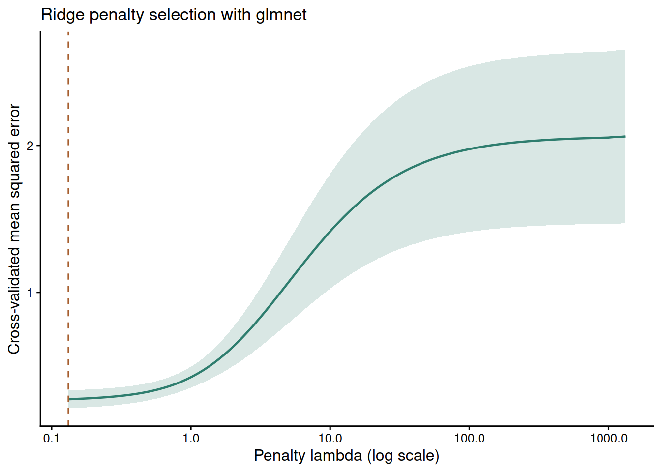
Choosing the Ridge Penalty with glmnet

The code below shows the same ridge idea using glmnet, which is the package readers are most likely to use in practice. The predictors are standardised internally, alpha = 0 requests ridge rather than lasso, and cross-validation selects a penalty. The sample is deliberately small, so the cross-validation curve should be read as a tuning aid rather than as a precise estimate of out-of-sample performance.

Rendered Output

Table 13.4

Ridge estimates from glmnet at the selected penalty

Term	Estimate
(Intercept)	2.183
wait_time	-0.180
friendliness	0.740

Note. The selected lambda is the value minimising cross-validated prediction error. In small samples, repeat the analysis under plausible modelling choices rather than treating one cross-validation split as definitive.

Cell Code

Figure 13.2: Cross-validation curve for ridge penalty selection with glmnet.

LASSO for Predictor Screening

The LASSO uses an L1 penalty rather than the squared L2 penalty used by ridge regression. This means that, as the penalty increases, some coefficients can be shrunk exactly to zero. That property makes LASSO useful for cautious predictor screening when a small dataset contains more candidate predictors than the sample can estimate reliably. It should not be treated as proof that excluded variables are irrelevant. With small samples, selected predictors can change under modest resampling or under a different set of candidate variables.

The example below uses 30 observations and five candidate predictors. Cross-validation chooses two common penalty values: lambda.min, which minimises the cross-validated error, and lambda.1se, which chooses a more parsimonious model within one standard error of that minimum.

Table 13.5

LASSO coefficients under two cross-validated penalty choices

Term	lambda.min	lambda.1se
Intercept	60.21	60.30
Service quality	3.10	2.27
Response speed	-1.61	-1.08
Price fairness	-0.81	0.00
Staff training	1.14	0.06
Waiting-room comfort	-0.19	0.00

Note. Coefficients were estimated with standardised predictors. Values equal to 0 indicate variables removed by the LASSO penalty at that tuning value.

Figure 13.3: LASSO coefficient paths for five candidate predictors.

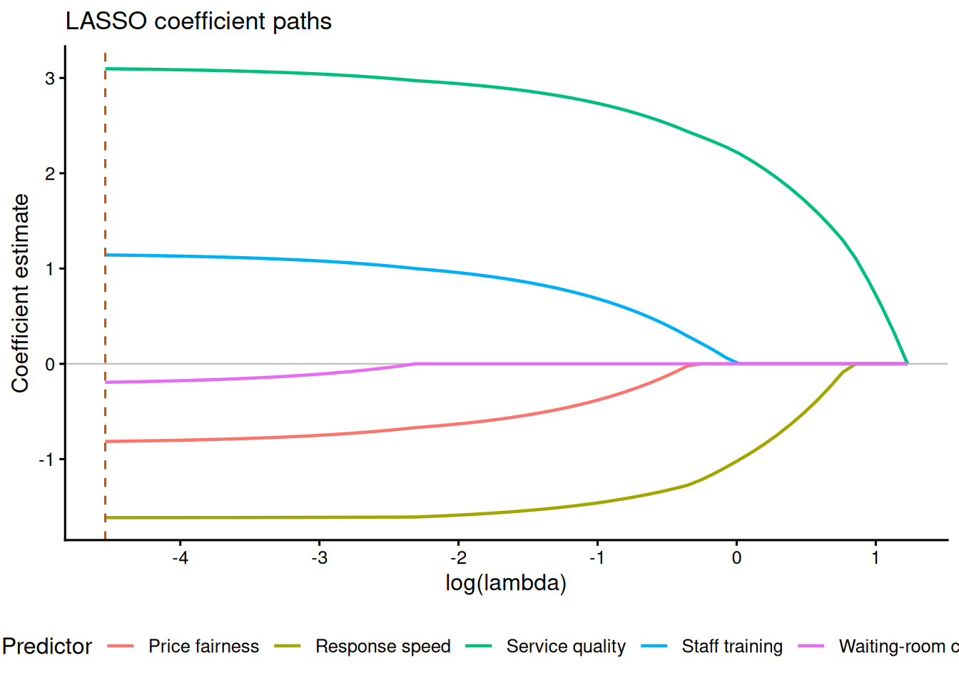
The main reporting point is the penalty rule, not just the final coefficients. If lambda.1se removes a predictor that lambda.min retains, describe that predictor as unstable rather than definitively absent. For explanatory work, LASSO is best used as a sensitivity analysis or screening tool before a simpler, pre-specified model is reported.

Bayesian Priors as Regularisation

Weakly informative priors are regularisation tools, not a way to force a preferred conclusion. A prior such as Normal(0, 2.5) on a logistic-regression coefficient implies that odds ratios between exp(-5) = 0.007 and exp(5) = 148 are plausible a priori while still regularising extreme estimates. Stronger priors such as Normal(0, 0.5) exert more shrinkage and should be justified by substantive knowledge or prior evidence (Gelman, Simpson, and Betancourt 2017).

Table 13.6 illustrates prior sensitivity for the wait-time slope in the customer-satisfaction example using a normal approximation to the likelihood. The table is not a replacement for full Bayesian computation, but it shows the main principle: when the prior is tight, the posterior moves toward zero. When the prior is weak, the posterior resembles the data-driven estimate.

Table 13.6

Prior-sensitivity illustration for a Bayesian regression slope

Prior on wait-time slope	Posterior mean	Posterior SD	95% credible interval
Normal(0, 0.5)	-0.17	0.27	-0.69 to 0.36
Normal(0, 1)	-0.21	0.30	-0.81 to 0.38
Normal(0, 2.5)	-0.23	0.32	-0.85 to 0.39
Normal(0, 10)	-0.24	0.32	-0.86 to 0.39

Note. The approximation uses the ordinary least-squares wait-time slope and standard error as a normal likelihood. Full Bayesian analyses should still check convergence diagnostics, such as R-hat < 1.01 and effective sample size > 400, and should inspect posterior predictive fit.

For a full Bayesian fit, use an MCMC package and report diagnostics. The following code is intentionally not evaluated in the book render because brms requires a working Stan toolchain, but it is the minimal workflow expected in a manuscript: specify priors, sample, check R-hat and effective sample size, and inspect posterior predictive fit. Before running it locally, verify the Stan toolchain with cmdstanr::check_cmdstan_toolchain() if using CmdStan, or confirm the installed rstan version with rstan::stan_version() before fitting a small test model.

Bayesian regression reports posterior intervals rather than frequentist confidence intervals. A 95% credible interval describes the range containing 95% of posterior probability given the model, data, and priors. That statement is conditional on the prior choice, so small-sample Bayesian reports should include the priors, convergence diagnostics, posterior predictive checks, and at least one plausible prior-sensitivity analysis. For leave-one-out cross-validation or WAIC in Bayesian models, use them as approximate predictive checks, not as automatic proof that one small-sample model is correct (Vehtari, Gelman, and Gabry 2017).

Reporting Regularised Models

A regularised model report should make the stabilising assumption visible. State the outcome, sample size, event count where relevant, candidate predictors, standardisation, penalty or prior, tuning method and sensitivity checks. Do not report a penalised coefficient as if it were an ordinary unpenalised estimate.

For Firth logistic regression, report the sparse event table, the separation warning or diagnostic that motivated the method, coefficient scale, odds ratios if used, confidence intervals and software. For ridge and LASSO, report whether predictors were standardised, the value of lambda, how lambda was chosen, and whether conclusions change under lambda.min versus lambda.1se or under a simpler unpenalised model. For Bayesian models, report priors, seed, chains, iterations, R-hat, effective sample size, posterior intervals and posterior predictive checks.

A concise reporting sentence could read: “Because the ordinary logistic model produced fitted probabilities close to 0 and 1, we estimated a Firth-penalised logistic regression. The model included planning score and prior experience, reported coefficients on the log-odds scale with confidence intervals, and was interpreted as a stabilised sensitivity analysis rather than as precise evidence from a large sample.” That level of detail is enough for readers to see both the method and the limitation.

Key Takeaways

Penalised and Bayesian regression methods are valuable in small samples because they make unstable estimates finite and reduce overfitting. Firth logistic regression is especially useful for sparse binary outcomes and separation. Ridge regression shrinks correlated or noisy linear-model coefficients. LASSO can screen candidate predictors by setting unstable coefficients to zero. Bayesian priors regularise estimates and express assumptions directly. The reporting obligation is the same in all cases: show the data structure, state the penalty or prior, check sensitivity, and avoid treating regularised estimates as more precise than the sample supports.

Self-Assessment Quiz

Question 1. What does separation mean in logistic regression?

Predictors are measured on different scalesA predictor or predictor combination nearly perfectly classifies the binary outcomeThe residuals are normally distributedThe model has no intercept

Explanation.

Separation occurs when the outcome can be nearly or perfectly predicted from the covariates. Standard logistic maximum likelihood can then produce extremely large or infinite coefficients.

Question 2. Why is Firth logistic regression useful with sparse binary outcomes?

It removes the binary outcomeIt reduces small-sample bias and produces finite estimates under separationIt guarantees statistical significanceIt replaces the need to report event counts

Explanation.

Firth’s method uses a penalised likelihood that reduces small-sample bias and avoids infinite estimates. Event counts and uncertainty still need to be reported.

Question 3. What does ridge regression do to coefficients?

It forces all coefficients to be exactly zeroIt shrinks coefficients toward zero by penalising large valuesIt converts a binary outcome into a countIt removes the need to standardise predictors

Explanation.

Ridge regression adds a squared-coefficient penalty. Larger penalties pull estimates toward zero and can reduce overfitting.

Question 4. In a small-sample Bayesian regression, why should prior sensitivity be reported?

Because priors have no effectBecause small samples can leave the posterior sensitive to reasonable prior choicesBecause it replaces convergence diagnosticsBecause credible intervals are always narrow

Explanation.

When the data are thin, different plausible priors can lead to noticeably different posterior estimates. Reporting sensitivity shows how much the conclusion depends on modelling assumptions.

Question 5. Which statement is the safest interpretation of a regularised estimate?

It is automatically unbiasedIt is stabilised by an explicit penalty or prior and should be interpreted with that assumption statedIt proves that the effect existsIt needs no confidence or credible interval

Explanation.

Regularisation stabilises estimates by adding assumptions. Those assumptions, along with intervals and diagnostics, must be reported.

Ayre, Colin, and Andrew J. Scally. 2014. ‘Critical Values for Lawshe’s Content Validity Ratio: Revisiting the Original Methods of Calculation’. Measurement and Evaluation in Counseling and Development 47 (1): 79–86. https://doi.org/10.1177/0748175613513808.

Briggs, Steven R., and Jonathan M. Cheek. 1986. ‘The Role of Factor Analysis in the Development and Evaluation of Personality Scales’. Journal of Personality 54 (1): 106–48.

Buuren, Stef van. 2018. Flexible Imputation of Missing Data. 2nd ed. Boca Raton, FL: Chapman; Hall/CRC.

Cameron, A. Colin, and Pravin K. Trivedi. 2013. Regression Analysis of Count Data. 2nd ed. Cambridge: Cambridge University Press. https://doi.org/10.1017/CBO9781139013567.

Chen, Henian, Patricia Cohen, and Sophie Chen. 2010. ‘How Big Is a Big Odds Ratio? Interpreting the Magnitudes of Odds Ratios in Epidemiological Studies’. Communications in Statistics - Simulation and Computation 39 (4): 860–64. https://doi.org/10.1080/03610911003650383.

Cicchetti, Domenic V. 1994. ‘Guidelines, Criteria, and Rules of Thumb for Evaluating Normed and Standardized Assessment Instruments in Psychology’. Psychological Assessment 6 (4): 284–90. https://doi.org/10.1037/1040-3590.6.4.284.

Clark, Lee Anna, and David Watson. 1995. ‘Constructing Validity: Basic Issues in Objective Scale Development’. Psychological Assessment 7 (3): 309–19.

Cohen, Jacob. 1988. Statistical Power Analysis for the Behavioral Sciences. 2nd ed. Hillsdale, NJ: Lawrence Erlbaum Associates.

Conover, W. J. 1999. Practical Nonparametric Statistics. 3rd ed. New York: John Wiley & Sons.

Costello, Anna B., and Jason Osborne. 2005. ‘Best Practices in Exploratory Factor Analysis: Four Recommendations for Getting the Most from Your Analysis’. Practical Assessment, Research, and Evaluation 10 (1): 1–9. https://doi.org/10.7275/jyj1-4868.

Davison, A. C., and D. V. Hinkley. 1997. Bootstrap Methods and Their Application. Cambridge Series in Statistical and Probabilistic Mathematics. Cambridge: Cambridge University Press.

DeVellis, Robert F., and Carolyn T. Thorpe. 2021. Scale Development: Theory and Applications. 5th ed. Thousand Oaks, CA: SAGE Publications.

Dienes, Zoltan. 2014. ‘Using Bayes to Get the Most Out of Non-Significant Results’. Frontiers in Psychology 5: 781. https://doi.org/10.3389/fpsyg.2014.00781.

Efron, Bradley, and Robert J. Tibshirani. 1993. An Introduction to the Bootstrap. New York, NY: Chapman; Hall/CRC.

Elm, Erik von, Douglas G. Altman, Matthias Egger, Stuart J. Pocock, Peter C. Gøtzsche, and Jan P. Vandenbroucke. 2007. ‘The Strengthening the Reporting of Observational Studies in Epidemiology (STROBE) Statement: Guidelines for Reporting Observational Studies’. PLoS Medicine 4 (10): e296. https://doi.org/10.1371/journal.pmed.0040296.

Fay, Michael P. 2010. ‘Confidence Intervals That Match Fisher’s Exact or Blaker’s Exact Tests’. Biostatistics 11 (2): 373–74. https://doi.org/10.1093/biostatistics/kxp050.

Firth, David. 1993. ‘Bias Reduction of Maximum Likelihood Estimates’. Biometrika 80 (1): 27–38. https://doi.org/10.1093/biomet/80.1.27.

Gelman, Andrew, Daniel Simpson, and Michael Betancourt. 2017. ‘The Prior Can Often Only Be Understood in the Context of the Likelihood’. Entropy 19 (10): 555. https://doi.org/10.3390/e19100555.

Good, Phillip I. 2005. Permutation, Parametric, and Bootstrap Tests of Hypotheses. 3rd ed. New York: Springer.

Graham, John W. 2009. ‘Missing Data Analysis: Making It Work in the Real World’. Annual Review of Psychology 60: 549–76. https://doi.org/10.1146/annurev.psych.58.110405.085530.

Hair, Joseph F., G. Tomas M. Hult, Christian M. Ringle, and Marko Sarstedt. 2017. A Primer on Partial Least Squares Structural Equation Modeling (PLS-SEM). 2nd ed. Thousand Oaks, CA: SAGE Publications.

Harrell, Frank E. 2015. Regression Modeling Strategies: With Applications to Linear Models, Logistic and Ordinal Regression, and Survival Analysis. 2nd ed. Springer Series in Statistics. New York: Springer. https://doi.org/10.1007/978-3-319-19425-7.

Heinze, Georg, and Michael Schemper. 2002. ‘A Solution to the Problem of Separation in Logistic Regression’. Statistics in Medicine 21 (16): 2409–19. https://doi.org/10.1002/sim.1047.

Hodges, Jr., J. L., and E. L. Lehmann. 1963. ‘Estimates of Location Based on Rank Tests’. The Annals of Mathematical Statistics 34 (2): 598–611. https://doi.org/10.1214/aoms/1177704172.

Hoenig, John M., and Dennis M. Heisey. 2001. ‘The Abuse of Power: The Pervasive Fallacy of Power Calculations for Data Analysis’. The American Statistician 55 (1): 19–24.

Hosmer, David W., Stanley Lemeshow, and Rodney X. Sturdivant. 2013. Applied Logistic Regression. 3rd ed. Wiley Series in Probability and Statistics. Hoboken, NJ: John Wiley & Sons. https://doi.org/10.1002/9781118548387.

Hu, Li-tze, and Peter M. Bentler. 1999. ‘Cutoff Criteria for Fit Indexes in Covariance Structure Analysis: Conventional Criteria Versus New Alternatives’. Structural Equation Modeling 6 (1): 1–55. https://doi.org/10.1080/10705519909540118.

Huberty, Carl J., and Stephen Olejnik. 2006. Applied MANOVA and Discriminant Analysis. 2nd ed. Hoboken, NJ: Wiley. https://doi.org/10.1002/047178947X.

Hwang, Ching-Lai, and Kwangsun Yoon. 1981. Multiple Attribute Decision Making: Methods and Applications. Berlin: Springer. https://doi.org/10.1007/978-3-642-48318-9.

Hyndman, Rob J., and George Athanasopoulos. 2021. Forecasting: Principles and Practice. 3rd ed. Melbourne, Australia: OTexts. https://otexts.com/fpp3/.

Koo, Terry K., and Mae Y. Li. 2016. ‘A Guideline of Selecting and Reporting Intraclass Correlation Coefficients for Reliability Research’. Journal of Chiropractic Medicine 15 (2): 155–63. https://doi.org/10.1016/j.jcm.2016.02.012.

Kraft, Matthew A. 2020. ‘Interpreting Effect Sizes of Education Interventions’. Educational Researcher 49 (4): 241–53. https://doi.org/10.3102/0013189X20912798.

Lakens, Daniël. 2013. ‘Calculating and Reporting Effect Sizes to Facilitate Cumulative Science: A Practical Primer for t-Tests and ANOVAs’. Frontiers in Psychology 4: 863. https://doi.org/10.3389/fpsyg.2013.00863.

Lakens, Daniël, Anne M. Scheel, and Peder M. Isager. 2018. ‘Equivalence Testing for Psychological Research: A Tutorial’. Advances in Methods and Practices in Psychological Science 1 (2): 259–69. https://doi.org/10.1177/2515245918770963.

Lawshe, Charles H. 1975. ‘A Quantitative Approach to Content Validity’. Personnel Psychology 28 (4): 563–75. https://doi.org/10.1111/j.1744-6570.1975.tb01393.x.

Lipsey, Mark W., and David B. Wilson. 1993. ‘The Efficacy of Psychological, Educational, and Behavioural Treatment: Confirmation from Meta-Analysis’. American Psychologist 48 (12): 1181–1209. https://doi.org/10.1037/0003-066X.48.12.1181.

Little, Roderick J. A. 1988. ‘A Test of Missing Completely at Random for Multivariate Data with Missing Values’. Journal of the American Statistical Association 83 (404): 1198–1202. https://doi.org/10.1080/01621459.1988.10478722.

MacKinnon, David P., Jennifer L. Krull, and Chondra M. Lockwood. 2000. ‘Equivalence of the Mediation, Confounding and Suppression Effect’. Prevention Science 1 (4): 173–81.

Mair, Patrick, and Rand R. Wilcox. 2020. ‘Robust Statistical Methods in r Using the WRS2 Package’. Behavior Research Methods 52 (2): 464–88. https://doi.org/10.3758/s13428-019-01246-w.

Mann, Henry B., and Donald R. Whitney. 1947. ‘On a Test of Whether One of Two Random Variables Is Stochastically Larger Than the Other’. The Annals of Mathematical Statistics 18 (1): 50–60. https://doi.org/10.1214/aoms/1177730491.

McDonald, Roderick P. 1999. Test Theory: A Unified Treatment. Mahwah, NJ: Lawrence Erlbaum Associates.

Morey, Richard D., and Jeffrey N. Rouder. 2011. ‘Bayes Factor Approaches for Testing Interval Null Hypotheses’. Psychological Methods 16 (4): 406–19. https://doi.org/10.1037/a0024377.

Nielsen, Jakob. 1993. Usability Engineering. San Francisco, CA: Morgan Kaufmann.

Olsson, Ulf. 1979. ‘Maximum Likelihood Estimation of the Polychoric Correlation Coefficient’. Psychometrika 44 (4): 443–60.

Opricovic, Serafim, and Gwo-Hshiung Tzeng. 2004. ‘Compromise Solution by MCDM Methods: A Comparative Analysis of VIKOR and TOPSIS’. European Journal of Operational Research 156 (2): 445–55. https://doi.org/10.1016/S0377-2217(03)00020-1.

Page, Matthew J., Joanne E. McKenzie, Patrick M. Bossuyt, Isabelle Boutron, Tammy C. Hoffmann, Cynthia D. Mulrow, Larissa Shamseer, et al. 2021. ‘The PRISMA 2020 Statement: An Updated Guideline for Reporting Systematic Reviews’. BMJ 372: n71. https://doi.org/10.1136/bmj.n71.

R Core Team. 2026. R: A Language and Environment for Statistical Computing. Vienna, Austria: R Foundation for Statistical Computing. https://www.R-project.org/.

Rubin, Donald B. 1987. Multiple Imputation for Nonresponse in Surveys. New York, NY: Wiley.

Saaty, Thomas L. 1980. The Analytic Hierarchy Process. New York, NY: McGraw-Hill.

Schulz, Kenneth F., Douglas G. Altman, and David Moher. 2010. ‘CONSORT 2010 Statement: Updated Guidelines for Reporting Parallel Group Randomised Trials’. BMJ 340: c332. https://doi.org/10.1136/bmj.c332.

Shan, Guogen. 2018. Exact Statistical Inference for Categorical Data. London: Academic Press.

Sterne, Jonathan A. C., Ian R. White, John B. Carlin, Michael Spratt, Patrick Royston, Michael G. Kenward, Angela M. Wood, and James R. Carpenter. 2009. ‘Multiple Imputation for Missing Data in Epidemiological and Clinical Research: Potential and Pitfalls’. BMJ 338: b2393. https://doi.org/10.1136/bmj.b2393.

Teare, M. Dawn, Munyaradzi Dimairo, Neil Shephard, Amanda Hayman, Amy Whitehead, and Stephen J. Walters. 2014. ‘Sample Size Requirements to Estimate Key Design Parameters from External Pilot Randomised Controlled Trials: A Simulation Study’. Trials 15: 264. https://doi.org/10.1186/1745-6215-15-264.

Tomczak, Maciej, and Ewa Tomczak. 2014. ‘The Need to Report Effect Size Estimates Revisited: An Overview of Some Recommended Measures of Effect Size’. Trends in Sport Sciences 21 (1): 19–25.

Trizano-Hermosilla, Italo, and Jose M. Alvarado. 2016. ‘Best Alternatives to Cronbach’s Alpha Reliability in Realistic Conditions: Congeneric and Asymmetrical Measurements’. Frontiers in Psychology 7: 769. https://doi.org/10.3389/fpsyg.2016.00769.

Van de Schoot, Rens, and Milica Miočević. 2020. Small Sample Size Solutions: A Guide for Applied Researchers and Practitioners. London: Routledge.

Vehtari, Aki, Andrew Gelman, and Jonah Gabry. 2017. ‘Practical Bayesian Model Evaluation Using Leave-One-Out Cross-Validation and WAIC’. Statistics and Computing 27 (5): 1413–32. https://doi.org/10.1007/s11222-016-9696-4.

Wagenmakers, Eric-Jan, Jonathon Love, Maarten Marsman, Tahira Jamil, Alexander Ly, Josine Verhagen, Ravi Selker, et al. 2018. ‘Bayesian Inference for Psychology. Part II: Example Applications with JASP’. Psychonomic Bulletin & Review 25 (1): 58–76. https://doi.org/10.3758/s13423-017-1323-7.

White, Ian R., Patrick Royston, and Angela M. Wood. 2011. ‘Multiple Imputation Using Chained Equations: Issues and Guidance for Practice’. Statistics in Medicine 30 (4): 377–99. https://doi.org/10.1002/sim.4067.