Chapter 10: Exact Tests and Resampling Methods

Small-sample analysis often requires reference distributions that do not depend on large-sample theory.

Exact tests and resampling methods become especially useful when sample sizes are modest and large-sample approximations carry meaningful risk of inaccuracy. This chapter explains when to use exact tests for discrete outcomes, when permutation tests provide a cleaner reference distribution than a parametric model, and when bootstrap resampling is useful for interval estimation. The emphasis is practical: matching the method to the design, the outcome type, and the inferential goal.

Learning Objectives

By the end of this chapter, you will be able to explain when exact tests are preferable to large-sample approximations, distinguish conditional exact tests from unconditional and mid-p alternatives, implement exact binomial, exact Poisson, permutation, and bootstrap procedures in R, and report resampling analyses with enough detail for readers to reproduce the statistic, number of resamples, random seed, and inferential target.

When to Use Exact and Resampling Methods

Exact tests calculate p-values directly from the null distribution of the statistic. They are especially useful when the outcome is discrete, when expected cell counts are small, or when the sample is too limited for asymptotic results to be reliable.

Resampling methods use the observed data to approximate a sampling distribution. Permutation tests reassign labels under the null hypothesis to create a reference distribution for a test statistic. Bootstrap methods resample with replacement from the observed data to approximate the variability of an estimator and to construct confidence intervals.

In practice, exact tests are most natural for sparse binary or count data. Permutation tests are useful when exchangeability under the null is plausible. Bootstrap methods are especially helpful when the statistic of interest lacks a simple closed-form standard error.

For any resampling analysis, report the statistic being resampled and the number of permutations or bootstrap resamples. Also report the random seed and whether the result is exact or Monte Carlo. Those details determine the stability and reproducibility of the reported inference.

Fisher’s Exact Test for 2×2 Tables

Fisher’s exact test is the standard conditional test for association in a 2×2 contingency table when some expected cell counts are small. It conditions on the observed margins and calculates the probability of the observed table, and all equally or more extreme tables, under the null hypothesis of no association.

Because the sample space is discrete, Fisher’s test can be conservative: its p-value is guaranteed to control the Type I error rate, but that guarantee can come at the cost of reduced power. That trade-off is often acceptable in confirmatory work, especially when one of the margins is fixed by design.

Example: Fisher’s Exact Test

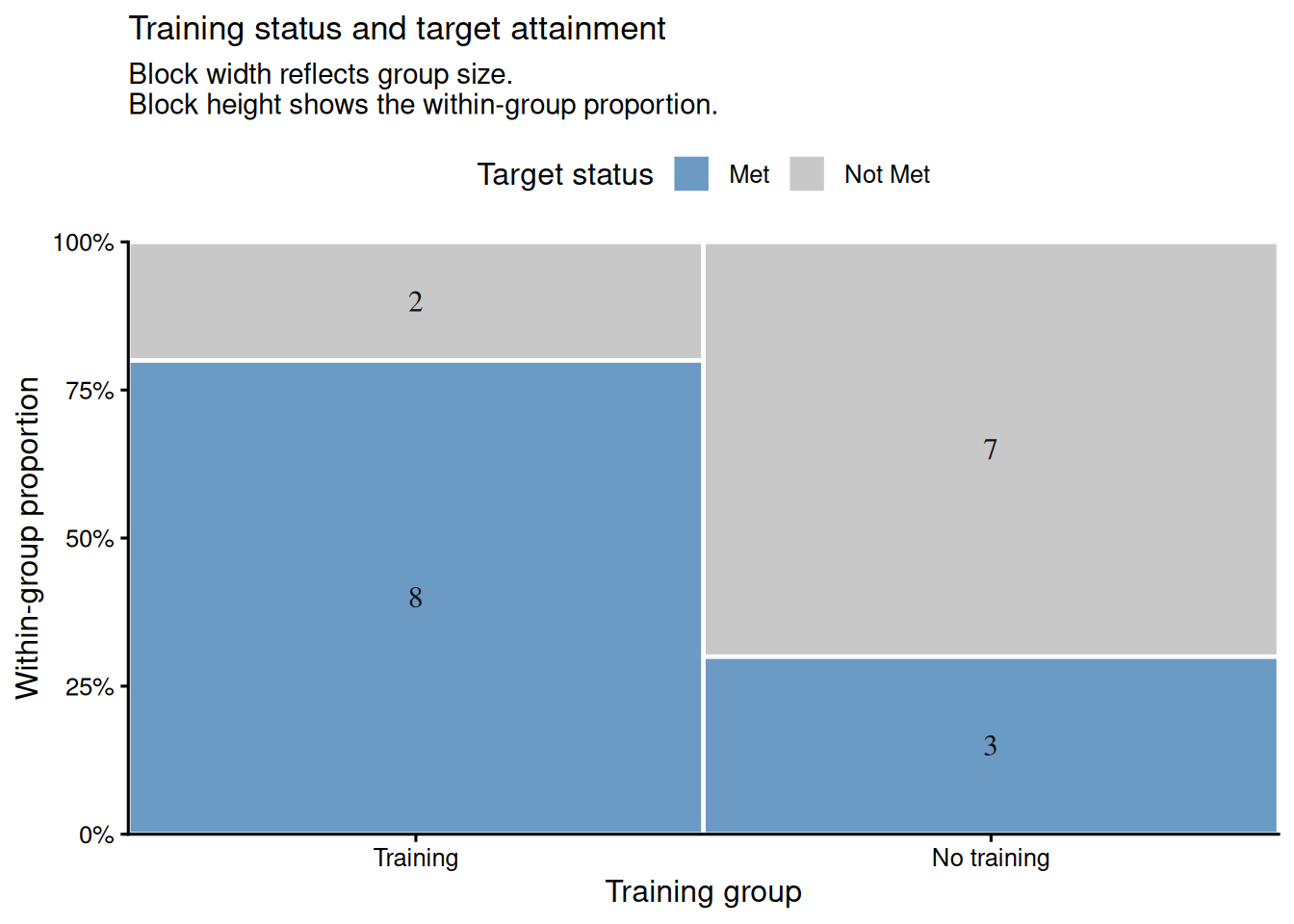
Suppose we are evaluating a new training intervention. Of 10 employees who received training, 8 met their performance target; of 10 who did not receive training, 3 met the target. We test whether training is associated with meeting the target.

Rendered Output

Table 10.1

Training outcomes by group

Training group	Met target	Did not meet target
Training	8	2
No training	3	7

Note. The smallest expected cell count under independence is 4.5, so exact inference is preferable to the chi-square approximation.

Cell Code

Fisher’s exact test gives an odds ratio of 8.15, with a 95% confidence interval from 0.88 to 127.06, and an exact two-sided p-value of 0.070. That odds ratio, despite the wide interval, points toward a meaningful association that a larger study would be well placed to assess.

Visualising the 2×2 Table

A mosaic-style plot helps readers see the same 2×2 structure graphically. The two training groups have equal width because each contains 10 employees, and the vertical split within each block shows the proportion who met the target. In this example, the training group has a visibly larger share of employees meeting the target.

Rendered Output

Figure 10.1: Mosaic-style plot of training status and target attainment. Block width reflects group size; block height within each group reflects the proportion meeting the target.

Cell Code

When Fisher’s Exact Test Is Conservative

Fisher’s exact test conditions on both row and column margins of the 2x2 table. In prospective studies, only the group sizes are fixed by design; conditioning on the observed outcome margin as well can make the test conservative. In case-control studies, both margins may align more closely with the sampling plan, though Fisher’s conditioning remains stricter than the design itself.

• Prospective study or trial: group sizes are fixed by design, so one margin matches the design directly. Fisher’s conditioning still also fixes the observed outcome margin, which is random and can make the test conservative.
• Case-control study: case and control totals are fixed by design, so the conditioning aligns more closely with the sampling plan, though Fisher’s exact conditioning is still stricter than the design itself.
• Cross-sectional or convenience sample: neither margin is fixed by design, so the extra conditioning is most visible and conservatism is often easiest to see.

The practical implication is straightforward: a Fisher p-value can stay above 0.05 even when a less conservative exact method gives stronger evidence. Fisher’s test remains valid, but the conditioning scheme affects how much power is available.

Unconditional Exact Tests

The unconditional approach, developed by Barnard, does not require conditioning on both margins. Modern implementations therefore offer unconditional exact tests that condition only on the group sizes. These tests are often more powerful than Fisher’s exact test when the margins are not fixed by design.

In R, the exact2x2 package provides unconditional exact procedures through uncondExact2x2() (Fay 2010). Install it with install.packages("exact2x2") if it is not already available. The score version shown below is Barnard-style in spirit and compares the observed proportions while conditioning only on the group sizes.

Rendered Output

Table 10.2

Comparison of exact p-values for the training example

Method	Conditioning	Two-sided p-value
Fisher's exact test	Conditions on both margins	0.070
Fisher's exact test with mid-p correction	Conditions on both margins, then applies a mid-p adjustment	0.038
Unconditional exact score test	Conditions on group sizes only	0.041

Note. The unconditional exact score test estimates a risk difference of 0.50, with a 95% confidence interval from 0.02 to 0.83.

Cell Code

For this table, Fisher’s exact p-value is 0.070, whereas the mid-p correction gives 0.038 and the unconditional exact score test gives 0.041. The unconditional method is less conservative here because it does not condition on both margins. Reported as training minus no training, the estimated risk difference is 0.50, with a 95% confidence interval from 0.02 to 0.83.

Mid-p Corrections

Mid-p corrections reduce conservatism by subtracting half the probability of the observed table from the tail area. This yields a test that does not guarantee Type I error control at the nominal level in every configuration. Report mid-p results as a sensitivity analysis alongside the standard Fisher test rather than as a replacement default.

WarningCommon Misconception: “Exact” Means “Automatically Best”

Myth: “If a test is exact, it must be the most appropriate or most informative option.”

Reality: Exactness describes how the p-value is computed under the null hypothesis. The appropriate conditioning scheme still depends on the design. In the training example above, Fisher’s exact test gives 0.070, while the mid-p and unconditional exact alternatives give 0.038 and 0.041 respectively.

Lesson:

1. Exact computation and design appropriateness are separate questions.
2. Fisher’s exact test is a strong default for confirmatory sparse 2×2 analyses.
3. Mid-p and unconditional exact tests are useful sensitivity checks when Fisher’s conditioning may be overly restrictive.
4. With very small samples, the effect estimate and the underlying table can be more informative than a p-value alone.

Exact Binomial Test

The exact binomial test assesses whether the observed number of successes is compatible with a hypothesised success probability. It is appropriate for a single binary outcome when the null benchmark is known in advance or supplied by design.

Example: Exact Binomial Test

A clinic claims that 70% of patients improve with standard care. In a small audit of 15 patients, 13 improved. We test whether the observed proportion is consistent with the clinic’s claim.

Rendered Output

Table 10.3

Exact binomial test summary

Observed successes	Observed proportion	Hypothesised proportion	95% exact CI	Exact p-value
13 of 15	0.867	0.70	0.60 to 0.98	0.258

Cell Code

The observed improvement proportion is 0.867, and the exact binomial p-value is 0.258. With such a small audit, the data remain compatible with the clinic’s claimed 70% rate. The 95% exact confidence interval from 0.60 to 0.98 is wide enough to include both the claimed value and substantially higher improvement rates.

Exact Poisson Test

The exact Poisson test is used for count data when the quantity of interest is the number of events in a fixed amount of time, area, or exposure. It tests whether an observed count is consistent with a specified Poisson rate.

Example: Exact Poisson Test

A manufacturing process is expected to produce 3 defects per batch on average. In a random sample of 8 batches, we observe 32 total defects. We test whether the observed rate is consistent with the expected rate of 3 per batch.

Rendered Output

Table 10.4

Exact Poisson test summary

Observed count	Observed rate	Hypothesised rate	95% exact CI	Exact p-value
32 defects across 8 batches	4.00 per batch	3.00 per batch	2.74 to 5.65	0.102

Cell Code

The observed defect rate is 4.00 per batch, compared with the hypothesised rate of 3.00. The exact Poisson p-value is 0.102, so the data are broadly consistent with the expected defect rate. The 95% exact interval from 2.74 to 5.65 still includes 3.00.

Permutation Tests

Permutation tests compare the observed statistic with the distribution obtained by rearranging group labels under the null hypothesis. When every possible reallocation is enumerated, the resulting p-value is exact under the null. When only a large random sample of reallocations is used, the result is a Monte Carlo approximation. For two groups of size n1 and n2, the number of reallocations is (n1 + n2)! / (n1! n2!), equivalent to choosing n1 observations from the pooled sample. If this number is computationally feasible, for example below 100,000, enumerate all permutations; otherwise use a large Monte Carlo sample such as B = 10,000 and report both B and the random seed.

The key assumption is exchangeability under the null hypothesis: if the null is true, the joint distribution of the data remains the same under any reassignment of labels. That makes permutation tests especially attractive for small-sample comparisons where a parametric model would be difficult to justify.

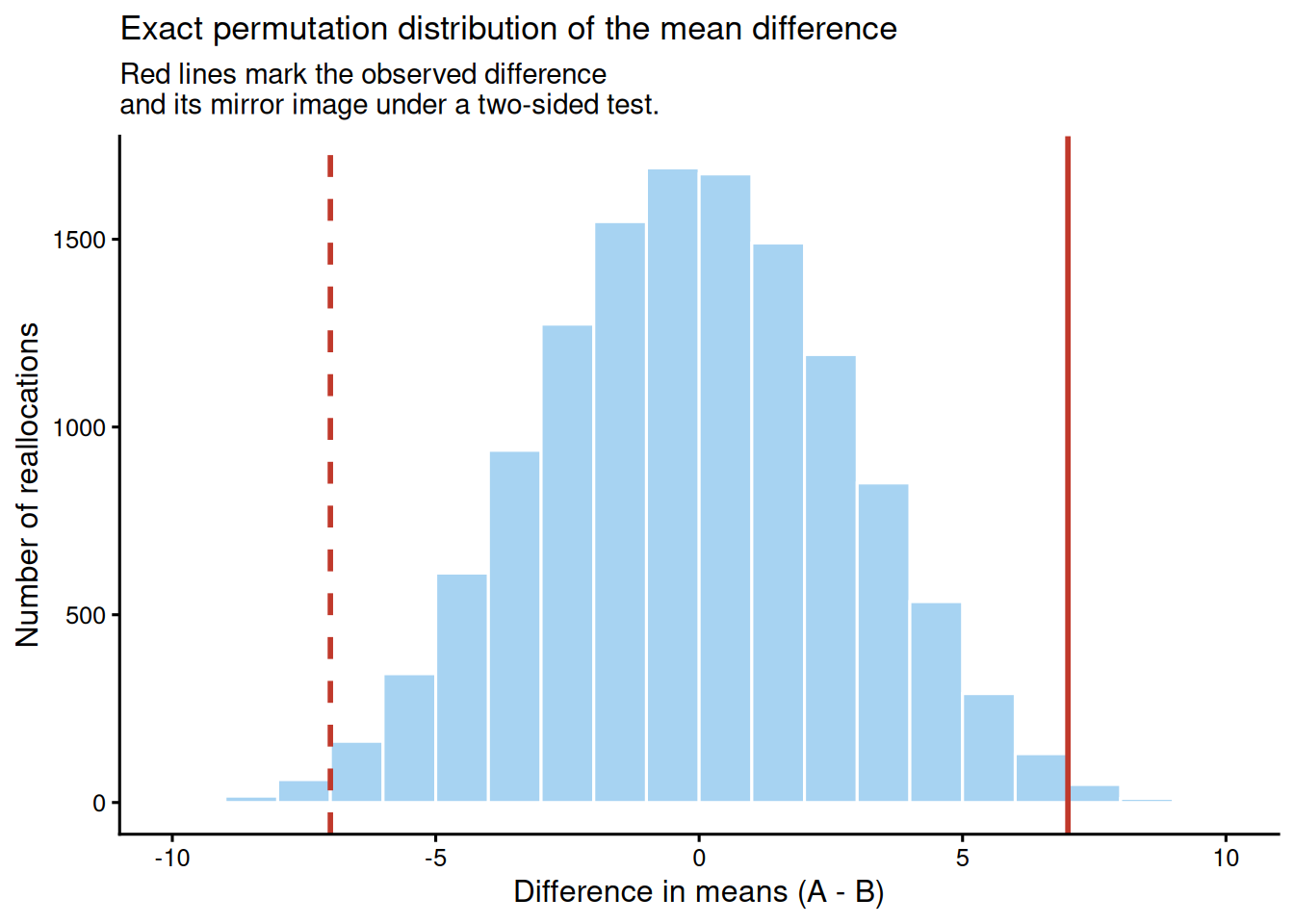
Example: Permutation Test for Difference in Means

We compare test scores between two teaching methods with small groups of 8 students each. The outcome is continuous, but with such a small sample it is reasonable to avoid normality assumptions and to test the mean difference by permutation.

Rendered Output

Figure 10.2: Exact permutation distribution for the mean difference between teaching methods.

Cell Code

Across all 12,870 possible reallocations, the observed mean difference is 7.00 points and the exact two-sided permutation p-value is 0.0126. Four-decimal precision is shown here because the exact enumeration produces a very small non-zero p-value. Because every possible label assignment is included, this result is exact rather than Monte Carlo. The figure makes the logic visible: the observed difference sits at the extreme tail of the permutation distribution.

Bootstrap Confidence Intervals

Bootstrap resampling constructs confidence intervals by repeatedly drawing samples with replacement from the observed data and recalculating the statistic of interest. The resulting bootstrap distribution approximates the sampling distribution of that statistic.

This chapter uses the nonparametric bootstrap, which resamples directly from the observed data. A parametric bootstrap simulates new datasets from a fitted parametric model, so its validity depends entirely on how well that model represents the data. For small-sample work, the nonparametric bootstrap is often the safer default when a model-free interval is desired.

Example: Bootstrap CI for the Median

We estimate the median recovery time for a small sample of patients and construct a 95% bootstrap confidence interval.

Rendered Output

Table 10.5

Bootstrap summary for median recovery time

Statistic	Estimate	95% percentile bootstrap CI	95% BCa bootstrap CI	Resamples
Median recovery time	16 days	14 to 17 days	14 to 17 days	2,000

Cell Code

The sample median recovery time is 16 days. The 95% percentile bootstrap interval runs from 14 to 17 days, and the BCa interval runs from 14 to 17 days. Both intervals summarise uncertainty around the median without requiring a normal-theory standard error formula. Percentile intervals are simple; BCa intervals adjust for bias and acceleration in the bootstrap distribution (Efron and Tibshirani 1993). With n < 30, BCa intervals can be unstable or fail when the statistic has many ties, so report the interval type and inspect the bootstrap distribution rather than treating BCa as automatically superior.

Key Takeaways

Exact tests are most valuable when the data are sparse enough that large-sample approximations become questionable. Fisher’s exact test is a strong default for sparse 2×2 tables, but mid-p and unconditional exact procedures can serve as useful sensitivity checks when Fisher’s conditioning is stronger than the design requires. Exact binomial and exact Poisson tests extend the same logic to single proportions and sparse event rates, while permutation tests rely on exchangeability and can be exact when every possible reallocation is enumerated. Bootstrap intervals are especially useful for statistics such as medians that lack simple analytic standard errors, provided the resampling procedure is reported transparently.

Self-Assessment Quiz

Test your understanding of exact tests and resampling methods from Chapter 10.

Question 1. When is Fisher’s exact test especially appropriate?

When every expected cell count is comfortably above 20When a 2×2 table has sparse counts and exact inference is preferredWhen the outcome is continuous and normally distributedWhen the goal is estimating a time-series trend

Explanation.

Fisher’s exact test is designed for sparse 2×2 tables where exact inference is preferred to the chi-square approximation. The chapter introduces it as the standard conditional test when some expected cell counts are small.

Question 2. Why can Fisher’s exact test be conservative in some settings?

It ignores the observed tableIt conditions on both margins, which can make rejection harder than necessary when both are not fixed by designIt always assumes normalityIt uses too many bootstrap resamples

Explanation.

The chapter explains that Fisher’s test conditions on both margins. When the design leaves one margin free, that conditioning can make the test more conservative and reduce power.

Question 3. When might Barnard-style unconditional tests or a mid-p correction be considered?

When you need a less conservative sensitivity check for sparse 2×2 dataWhen the outcome is continuous and homoscedasticWhen all expected counts exceed 100When fitting Bayesian regression with weakly informative priors

Explanation.

The chapter presents mid-p and unconditional exact procedures as less conservative alternatives or sensitivity checks for sparse 2×2 tables, especially when Fisher’s conditioning may be overly restrictive.

Question 4. What does the exact binomial test evaluate?

Whether two means differ after random permutationWhether an observed number of successes is consistent with a hypothesised proportionWhether a count process is overdispersed relative to PoissonWhether a regression model has converged

Explanation.

The exact binomial test is for a single-sample binary outcome. It compares the observed number of successes with a fixed benchmark proportion without relying on large-sample approximations.

Question 5. What is the exact Poisson test used for in this chapter?

Comparing two continuous variables with tied ranksTesting whether an observed event count or rate is consistent with a specified Poisson rateSelecting variables in penalised regressionChecking MCMC convergence

Explanation.

The chapter uses the exact Poisson test for sparse count data when the interest is whether an observed count or event rate differs from a known benchmark.

Question 6. What key assumption makes a permutation test valid under the null hypothesis?

Exchangeability of observations or labels under the nullNormal residuals with equal varianceAt least 100 observations per groupA Poisson-distributed outcome

Explanation.

Permutation tests rely on exchangeability under the null hypothesis. If the joint distribution of the data remains the same under any reassignment of labels, the permutation reference distribution is valid.

Question 7. Why is the bootstrap especially useful in small-sample work?

It guarantees narrow confidence intervalsIt can approximate uncertainty for statistics like medians when closed-form standard errors are unavailableIt removes the need to report uncertaintyIt is only valid for normal data

Explanation.

The bootstrap is useful when the statistic of interest does not have a simple analytic standard error or when a model-free interval is preferred. The chapter’s median example illustrates this directly.

Question 8. Which reporting detail is most important to include for resampling procedures?

Only whether the result was significantThe number of resamples or permutations, the statistic used, and enough detail to reproduce the procedureOnly the sample sizeOnly the largest resampled statistic

Explanation.

The chapter states that resampling analyses should report the statistic being resampled, the number of permutations or bootstrap resamples, the random seed, and whether the result is exact or Monte Carlo.

Ayre, Colin, and Andrew J. Scally. 2014. ‘Critical Values for Lawshe’s Content Validity Ratio: Revisiting the Original Methods of Calculation’. Measurement and Evaluation in Counseling and Development 47 (1): 79–86. https://doi.org/10.1177/0748175613513808.

Briggs, Steven R., and Jonathan M. Cheek. 1986. ‘The Role of Factor Analysis in the Development and Evaluation of Personality Scales’. Journal of Personality 54 (1): 106–48.

Buuren, Stef van. 2018. Flexible Imputation of Missing Data. 2nd ed. Boca Raton, FL: Chapman; Hall/CRC.

Cameron, A. Colin, and Pravin K. Trivedi. 2013. Regression Analysis of Count Data. 2nd ed. Cambridge: Cambridge University Press. https://doi.org/10.1017/CBO9781139013567.

Chen, Henian, Patricia Cohen, and Sophie Chen. 2010. ‘How Big Is a Big Odds Ratio? Interpreting the Magnitudes of Odds Ratios in Epidemiological Studies’. Communications in Statistics - Simulation and Computation 39 (4): 860–64. https://doi.org/10.1080/03610911003650383.

Cicchetti, Domenic V. 1994. ‘Guidelines, Criteria, and Rules of Thumb for Evaluating Normed and Standardized Assessment Instruments in Psychology’. Psychological Assessment 6 (4): 284–90. https://doi.org/10.1037/1040-3590.6.4.284.

Clark, Lee Anna, and David Watson. 1995. ‘Constructing Validity: Basic Issues in Objective Scale Development’. Psychological Assessment 7 (3): 309–19.

Cohen, Jacob. 1988. Statistical Power Analysis for the Behavioral Sciences. 2nd ed. Hillsdale, NJ: Lawrence Erlbaum Associates.

Conover, W. J. 1999. Practical Nonparametric Statistics. 3rd ed. New York: John Wiley & Sons.

Costello, Anna B., and Jason Osborne. 2005. ‘Best Practices in Exploratory Factor Analysis: Four Recommendations for Getting the Most from Your Analysis’. Practical Assessment, Research, and Evaluation 10 (1): 1–9. https://doi.org/10.7275/jyj1-4868.

Davison, A. C., and D. V. Hinkley. 1997. Bootstrap Methods and Their Application. Cambridge Series in Statistical and Probabilistic Mathematics. Cambridge: Cambridge University Press.

DeVellis, Robert F., and Carolyn T. Thorpe. 2021. Scale Development: Theory and Applications. 5th ed. Thousand Oaks, CA: SAGE Publications.

Dienes, Zoltan. 2014. ‘Using Bayes to Get the Most Out of Non-Significant Results’. Frontiers in Psychology 5: 781. https://doi.org/10.3389/fpsyg.2014.00781.

Efron, Bradley, and Robert J. Tibshirani. 1993. An Introduction to the Bootstrap. New York, NY: Chapman; Hall/CRC.

Elm, Erik von, Douglas G. Altman, Matthias Egger, Stuart J. Pocock, Peter C. Gøtzsche, and Jan P. Vandenbroucke. 2007. ‘The Strengthening the Reporting of Observational Studies in Epidemiology (STROBE) Statement: Guidelines for Reporting Observational Studies’. PLoS Medicine 4 (10): e296. https://doi.org/10.1371/journal.pmed.0040296.

Fay, Michael P. 2010. ‘Confidence Intervals That Match Fisher’s Exact or Blaker’s Exact Tests’. Biostatistics 11 (2): 373–74. https://doi.org/10.1093/biostatistics/kxp050.

Firth, David. 1993. ‘Bias Reduction of Maximum Likelihood Estimates’. Biometrika 80 (1): 27–38. https://doi.org/10.1093/biomet/80.1.27.

Gelman, Andrew, Daniel Simpson, and Michael Betancourt. 2017. ‘The Prior Can Often Only Be Understood in the Context of the Likelihood’. Entropy 19 (10): 555. https://doi.org/10.3390/e19100555.

Good, Phillip I. 2005. Permutation, Parametric, and Bootstrap Tests of Hypotheses. 3rd ed. New York: Springer.

Graham, John W. 2009. ‘Missing Data Analysis: Making It Work in the Real World’. Annual Review of Psychology 60: 549–76. https://doi.org/10.1146/annurev.psych.58.110405.085530.

Hair, Joseph F., G. Tomas M. Hult, Christian M. Ringle, and Marko Sarstedt. 2017. A Primer on Partial Least Squares Structural Equation Modeling (PLS-SEM). 2nd ed. Thousand Oaks, CA: SAGE Publications.

Harrell, Frank E. 2015. Regression Modeling Strategies: With Applications to Linear Models, Logistic and Ordinal Regression, and Survival Analysis. 2nd ed. Springer Series in Statistics. New York: Springer. https://doi.org/10.1007/978-3-319-19425-7.

Heinze, Georg, and Michael Schemper. 2002. ‘A Solution to the Problem of Separation in Logistic Regression’. Statistics in Medicine 21 (16): 2409–19. https://doi.org/10.1002/sim.1047.

Hodges, Jr., J. L., and E. L. Lehmann. 1963. ‘Estimates of Location Based on Rank Tests’. The Annals of Mathematical Statistics 34 (2): 598–611. https://doi.org/10.1214/aoms/1177704172.

Hoenig, John M., and Dennis M. Heisey. 2001. ‘The Abuse of Power: The Pervasive Fallacy of Power Calculations for Data Analysis’. The American Statistician 55 (1): 19–24.

Hosmer, David W., Stanley Lemeshow, and Rodney X. Sturdivant. 2013. Applied Logistic Regression. 3rd ed. Wiley Series in Probability and Statistics. Hoboken, NJ: John Wiley & Sons. https://doi.org/10.1002/9781118548387.

Hu, Li-tze, and Peter M. Bentler. 1999. ‘Cutoff Criteria for Fit Indexes in Covariance Structure Analysis: Conventional Criteria Versus New Alternatives’. Structural Equation Modeling 6 (1): 1–55. https://doi.org/10.1080/10705519909540118.

Huberty, Carl J., and Stephen Olejnik. 2006. Applied MANOVA and Discriminant Analysis. 2nd ed. Hoboken, NJ: Wiley. https://doi.org/10.1002/047178947X.

Hwang, Ching-Lai, and Kwangsun Yoon. 1981. Multiple Attribute Decision Making: Methods and Applications. Berlin: Springer. https://doi.org/10.1007/978-3-642-48318-9.

Hyndman, Rob J., and George Athanasopoulos. 2021. Forecasting: Principles and Practice. 3rd ed. Melbourne, Australia: OTexts. https://otexts.com/fpp3/.

Koo, Terry K., and Mae Y. Li. 2016. ‘A Guideline of Selecting and Reporting Intraclass Correlation Coefficients for Reliability Research’. Journal of Chiropractic Medicine 15 (2): 155–63. https://doi.org/10.1016/j.jcm.2016.02.012.

Kraft, Matthew A. 2020. ‘Interpreting Effect Sizes of Education Interventions’. Educational Researcher 49 (4): 241–53. https://doi.org/10.3102/0013189X20912798.

Lakens, Daniël. 2013. ‘Calculating and Reporting Effect Sizes to Facilitate Cumulative Science: A Practical Primer for t-Tests and ANOVAs’. Frontiers in Psychology 4: 863. https://doi.org/10.3389/fpsyg.2013.00863.

Lakens, Daniël, Anne M. Scheel, and Peder M. Isager. 2018. ‘Equivalence Testing for Psychological Research: A Tutorial’. Advances in Methods and Practices in Psychological Science 1 (2): 259–69. https://doi.org/10.1177/2515245918770963.

Lawshe, Charles H. 1975. ‘A Quantitative Approach to Content Validity’. Personnel Psychology 28 (4): 563–75. https://doi.org/10.1111/j.1744-6570.1975.tb01393.x.

Lipsey, Mark W., and David B. Wilson. 1993. ‘The Efficacy of Psychological, Educational, and Behavioural Treatment: Confirmation from Meta-Analysis’. American Psychologist 48 (12): 1181–1209. https://doi.org/10.1037/0003-066X.48.12.1181.

Little, Roderick J. A. 1988. ‘A Test of Missing Completely at Random for Multivariate Data with Missing Values’. Journal of the American Statistical Association 83 (404): 1198–1202. https://doi.org/10.1080/01621459.1988.10478722.

MacKinnon, David P., Jennifer L. Krull, and Chondra M. Lockwood. 2000. ‘Equivalence of the Mediation, Confounding and Suppression Effect’. Prevention Science 1 (4): 173–81.

Mair, Patrick, and Rand R. Wilcox. 2020. ‘Robust Statistical Methods in r Using the WRS2 Package’. Behavior Research Methods 52 (2): 464–88. https://doi.org/10.3758/s13428-019-01246-w.

Mann, Henry B., and Donald R. Whitney. 1947. ‘On a Test of Whether One of Two Random Variables Is Stochastically Larger Than the Other’. The Annals of Mathematical Statistics 18 (1): 50–60. https://doi.org/10.1214/aoms/1177730491.

McDonald, Roderick P. 1999. Test Theory: A Unified Treatment. Mahwah, NJ: Lawrence Erlbaum Associates.

Morey, Richard D., and Jeffrey N. Rouder. 2011. ‘Bayes Factor Approaches for Testing Interval Null Hypotheses’. Psychological Methods 16 (4): 406–19. https://doi.org/10.1037/a0024377.

Nielsen, Jakob. 1993. Usability Engineering. San Francisco, CA: Morgan Kaufmann.

Olsson, Ulf. 1979. ‘Maximum Likelihood Estimation of the Polychoric Correlation Coefficient’. Psychometrika 44 (4): 443–60.

Opricovic, Serafim, and Gwo-Hshiung Tzeng. 2004. ‘Compromise Solution by MCDM Methods: A Comparative Analysis of VIKOR and TOPSIS’. European Journal of Operational Research 156 (2): 445–55. https://doi.org/10.1016/S0377-2217(03)00020-1.

Page, Matthew J., Joanne E. McKenzie, Patrick M. Bossuyt, Isabelle Boutron, Tammy C. Hoffmann, Cynthia D. Mulrow, Larissa Shamseer, et al. 2021. ‘The PRISMA 2020 Statement: An Updated Guideline for Reporting Systematic Reviews’. BMJ 372: n71. https://doi.org/10.1136/bmj.n71.

R Core Team. 2026. R: A Language and Environment for Statistical Computing. Vienna, Austria: R Foundation for Statistical Computing. https://www.R-project.org/.

Rubin, Donald B. 1987. Multiple Imputation for Nonresponse in Surveys. New York, NY: Wiley.

Saaty, Thomas L. 1980. The Analytic Hierarchy Process. New York, NY: McGraw-Hill.

Schulz, Kenneth F., Douglas G. Altman, and David Moher. 2010. ‘CONSORT 2010 Statement: Updated Guidelines for Reporting Parallel Group Randomised Trials’. BMJ 340: c332. https://doi.org/10.1136/bmj.c332.

Shan, Guogen. 2018. Exact Statistical Inference for Categorical Data. London: Academic Press.

Sterne, Jonathan A. C., Ian R. White, John B. Carlin, Michael Spratt, Patrick Royston, Michael G. Kenward, Angela M. Wood, and James R. Carpenter. 2009. ‘Multiple Imputation for Missing Data in Epidemiological and Clinical Research: Potential and Pitfalls’. BMJ 338: b2393. https://doi.org/10.1136/bmj.b2393.

Teare, M. Dawn, Munyaradzi Dimairo, Neil Shephard, Amanda Hayman, Amy Whitehead, and Stephen J. Walters. 2014. ‘Sample Size Requirements to Estimate Key Design Parameters from External Pilot Randomised Controlled Trials: A Simulation Study’. Trials 15: 264. https://doi.org/10.1186/1745-6215-15-264.

Tomczak, Maciej, and Ewa Tomczak. 2014. ‘The Need to Report Effect Size Estimates Revisited: An Overview of Some Recommended Measures of Effect Size’. Trends in Sport Sciences 21 (1): 19–25.

Trizano-Hermosilla, Italo, and Jose M. Alvarado. 2016. ‘Best Alternatives to Cronbach’s Alpha Reliability in Realistic Conditions: Congeneric and Asymmetrical Measurements’. Frontiers in Psychology 7: 769. https://doi.org/10.3389/fpsyg.2016.00769.

Van de Schoot, Rens, and Milica Miočević. 2020. Small Sample Size Solutions: A Guide for Applied Researchers and Practitioners. London: Routledge.

Vehtari, Aki, Andrew Gelman, and Jonah Gabry. 2017. ‘Practical Bayesian Model Evaluation Using Leave-One-Out Cross-Validation and WAIC’. Statistics and Computing 27 (5): 1413–32. https://doi.org/10.1007/s11222-016-9696-4.

Wagenmakers, Eric-Jan, Jonathon Love, Maarten Marsman, Tahira Jamil, Alexander Ly, Josine Verhagen, Ravi Selker, et al. 2018. ‘Bayesian Inference for Psychology. Part II: Example Applications with JASP’. Psychonomic Bulletin & Review 25 (1): 58–76. https://doi.org/10.3758/s13423-017-1323-7.

White, Ian R., Patrick Royston, and Angela M. Wood. 2011. ‘Multiple Imputation Using Chained Equations: Issues and Guidance for Practice’. Statistics in Medicine 30 (4): 377–99. https://doi.org/10.1002/sim.4067.