```{r}
#| include: false
suppressPackageStartupMessages(library(tidyverse))
suppressPackageStartupMessages(library(knitr))
suppressPackageStartupMessages(library(htmltools))
suppressPackageStartupMessages(library(psych))
source(normalizePath(file.path(dirname(knitr::current_input(dir = TRUE)), "..", "R", "chapter_helpers.R"), mustWork = TRUE))
```
:::: {.content-visible when-format="html"}
```{webr-r}
#| context: setup
#| include: false
#| echo: false
library(dplyr)
library(ggplot2)
library(tidyr)
library(tibble)
library(purrr)
library(psych)
chapter6_scale_table <- function(number = NULL, title = NULL, data,
note = NULL,
align = rep("l", ncol(data)),
col.names = names(data),
digits = NULL) {
print(data)
invisible(data)
}
chapter6_simulate_scale <- function(n, loadings, noise_sd = 0.8, centre = 3,
prefix = "WRS", seed = 2025) {
set.seed(seed)
latent_score <- as.numeric(scale(rnorm(n)))
item_values <- purrr::map(
loadings,
~ round(pmin(pmax(centre + .x * latent_score + rnorm(n, 0, noise_sd), 1), 5))
)
names(item_values) <- paste0(prefix, seq_along(loadings))
tibble::as_tibble(item_values)
}
chapter6_problem_item_diagnostics <- function(data) {
alpha_result <- suppressWarnings(psych::alpha(data, warnings = FALSE, check.keys = FALSE))
r_cor <- stats::setNames(alpha_result$item.stats[, "r.cor"], rownames(alpha_result$item.stats))
tibble::tibble(
Item = names(data),
`Item-total r` = unname(r_cor[names(data)]),
Mean = purrr::map_dbl(data, mean),
SD = purrr::map_dbl(data, stats::sd),
`Extreme %` = 100 * purrr::map_dbl(data, ~ max(mean(.x == 1), mean(.x == 5)))
) |>
dplyr::mutate(
`Item-total r` = round(`Item-total r`, 2),
Mean = round(Mean, 2),
SD = round(SD, 2),
`Extreme %` = round(`Extreme %`, 0),
Flag = dplyr::case_when(
`Extreme %` >= 80 ~ "Ceiling/floor effect",
SD < 0.5 ~ "Low variance",
is.na(`Item-total r`) | `Item-total r` < 0.30 ~ "Weak correlation",
TRUE ~ "OK"
)
)
}
chapter6_reliability_summary <- function(data, nboot = 1000, seed = 2025) {
alpha_result <- suppressWarnings(psych::alpha(data, warnings = FALSE, check.keys = FALSE))
split_half <- psych::splitHalf(data)
old_seed <- if (exists(".Random.seed", envir = .GlobalEnv, inherits = FALSE)) {
get(".Random.seed", envir = .GlobalEnv)
} else {
NULL
}
on.exit({
if (is.null(old_seed)) {
if (exists(".Random.seed", envir = .GlobalEnv, inherits = FALSE)) {
rm(".Random.seed", envir = .GlobalEnv)
}
} else {
assign(".Random.seed", old_seed, envir = .GlobalEnv)
}
}, add = TRUE)
set.seed(seed)
alpha_boot <- replicate(nboot, {
idx <- sample(seq_len(nrow(data)), replace = TRUE)
suppressWarnings(psych::alpha(data[idx, , drop = FALSE], warnings = FALSE, check.keys = FALSE)$total$raw_alpha)
})
alpha_ci <- stats::quantile(
alpha_boot[is.finite(alpha_boot)],
probs = c(0.025, 0.975),
names = FALSE,
na.rm = TRUE
)
if (length(alpha_ci) < 2) {
alpha_ci <- c(NA_real_, NA_real_)
}
tibble::tibble(
Metric = c(
"Cronbach's alpha",
"Bootstrap 95% CI lower",
"Bootstrap 95% CI upper",
"Average inter-item correlation",
"Mean split-half reliability",
"Minimum split-half reliability",
"Maximum split-half reliability"
),
Value = c(
alpha_result$total$raw_alpha,
alpha_ci[1],
alpha_ci[2],
alpha_result$total$average_r,
split_half$meanr,
split_half$minrb,
split_half$maxrb
)
) |>
dplyr::mutate(Value = round(Value, 3))
}
```
::::
# Chapter 6: Developing Short Scales for Small Samples
### Learning Objectives
By the end of this chapter, you will be able to explain why short-scale development with small samples requires staged validation rather than one definitive study, match psychometric tools to the sample sizes they can realistically support, use item-level diagnostics to refine candidate items, and report scale-development evidence transparently without overstating what a pilot can show.
### The Scale Development Lifecycle
Scale development is inherently a multi-stage process. With small samples, researchers must be strategic about which psychometric analyses to conduct at each stage and which to reserve for later validation.
The small helper functions used below (for example, `chapter6_simulate_scale()` and `chapter6_problem_item_diagnostics()`) are defined in `R/chapter_helpers.R` and sourced in the setup chunk. Readers who want to run individual chunks can first run `source("R/chapter_helpers.R")` from the project root.
### The Iterative Process
#### Stage 1: Item Generation (n = 5–10 cognitive interviews)
A first round of about 5 to 10 cognitive interviews usually surfaces the clearest wording and comprehension problems in an initial item pool [@nielsen1993].
**Goal**: Generate a pool of 2–3× your target number of items and ensure they are comprehensible.
**Methods**:
- **Literature review**: Identify existing scales and adapt items
- **Expert consultation**: Subject matter experts suggest relevant content
- **Cognitive interviews**: Think-aloud protocols with 5–10 participants from the target population
**Example**:
:::: {.content-visible when-format="html"}
::::: {.panel-tabset group="part-c-analysis-methods-chapter-6-5-developing-short-scales-for-small-samples-cell-1"}
#### Rendered Output
```{r}
#| label: part-c-scale-dev-1-html
#| echo: false
#| results: asis
item_pool <- tibble(
item_id = 1:15,
item_text = c(
"I feel confident handling work challenges",
"I bounce back quickly from setbacks",
"I maintain composure under pressure",
"I remain calm when facing obstacles",
"I trust my ability to solve problems",
"I recover from stress effectively",
"I rebound after difficult situations",
"I regain focus after disruptions",
"I process setbacks constructively",
"I maintain perspective during challenges",
"I adapt easily to changing priorities",
"I adjust my approach when needed",
"I seek support when needed",
"I learn from difficult experiences",
"I embrace new work demands"
),
domain = rep(c("Confidence", "Recovery", "Adaptability"), each = 5),
cognitive_issues = c(
NA, "Ambiguous: what counts as 'quickly'?", NA, NA, NA,
NA, "Too similar to item 2", NA, NA, NA,
NA, NA, "Double-barreled: 'seek' and 'support'", NA, NA
)
)
chapter6_scale_table(
number = "6.1",
title = "Candidate items flagged during cognitive interviewing.",
data = item_pool %>%
dplyr::filter(!is.na(cognitive_issues)) %>%
dplyr::transmute(
`Item ID` = item_id,
`Candidate Item` = item_text,
`Interview Note` = cognitive_issues
),
note = "Items flagged during think-aloud work should be revised before any pilot administration.",
align = c("r", "l", "l")
)
```
#### Cell Code
```{webr-r}
#| context: interactive
# Documenting item generation
item_pool <- tibble(
item_id = 1:15,
item_text = c(
"I feel confident handling work challenges",
"I bounce back quickly from setbacks",
"I maintain composure under pressure",
"I remain calm when facing obstacles",
"I trust my ability to solve problems",
"I recover from stress effectively",
"I rebound after difficult situations",
"I regain focus after disruptions",
"I process setbacks constructively",
"I maintain perspective during challenges",
"I adapt easily to changing priorities",
"I adjust my approach when needed",
"I seek support when needed",
"I learn from difficult experiences",
"I embrace new work demands"
),
domain = rep(c("Confidence", "Recovery", "Adaptability"), each = 5),
cognitive_issues = c(
NA, "Ambiguous: what counts as 'quickly'?", NA, NA, NA,
NA, "Too similar to item 2", NA, NA, NA,
NA, NA, "Double-barreled: 'seek' and 'support'", NA, NA
)
)
chapter6_scale_table(
number = "6.1",
title = "Candidate items flagged during cognitive interviewing.",
data = item_pool %>%
dplyr::filter(!is.na(cognitive_issues)) %>%
dplyr::transmute(
`Item ID` = item_id,
`Candidate Item` = item_text,
`Interview Note` = cognitive_issues
),
note = "Items flagged during think-aloud work should be revised before any pilot administration.",
align = c("r", "l", "l")
)
```
:::::
::::
:::: {.content-visible unless-format="html"}
```{r}
#| label: part-c-scale-dev-1
#| results: asis
item_pool <- tibble(
item_id = 1:15,
item_text = c(
"I feel confident handling work challenges",
"I bounce back quickly from setbacks",
"I maintain composure under pressure",
"I remain calm when facing obstacles",
"I trust my ability to solve problems",
"I recover from stress effectively",
"I rebound after difficult situations",
"I regain focus after disruptions",
"I process setbacks constructively",
"I maintain perspective during challenges",
"I adapt easily to changing priorities",
"I adjust my approach when needed",
"I seek support when needed",
"I learn from difficult experiences",
"I embrace new work demands"
),
domain = rep(c("Confidence", "Recovery", "Adaptability"), each = 5),
cognitive_issues = c(
NA, "Ambiguous: what counts as 'quickly'?", NA, NA, NA,
NA, "Too similar to item 2", NA, NA, NA,
NA, NA, "Double-barreled: 'seek' and 'support'", NA, NA
)
)
chapter6_scale_table(
number = "6.1",
title = "Candidate items flagged during cognitive interviewing.",
data = item_pool %>%
dplyr::filter(!is.na(cognitive_issues)) %>%
dplyr::transmute(
`Item ID` = item_id,
`Candidate Item` = item_text,
`Interview Note` = cognitive_issues
),
note = "Items flagged during think-aloud work should be revised before any pilot administration.",
align = c("r", "l", "l")
)
```
::::
**Key Point**: At this stage, **do NOT collect quantitative data**. Focus on qualitative feedback about item clarity, relevance, and comprehensiveness.
#### Stage 2: Pilot Testing (n = 20–30)
**Goal**: Identify problematic items before committing to a larger study.
**Methods**:
- Administer all items to a small pilot sample
- Compute **item-total correlations** (r.cor)
- Check for **ceiling/floor effects** (> 80% at extreme response)
- Examine **item means and SDs** (avoid items with no variance)
**What you CAN do with n = 20–30**:
At this stage, item-total correlations are screening tools rather than definitive item-deletion criteria. With `n = 20–30`, values near the usual `0.30` heuristic have substantial sampling variability, so a result like `0.28` versus `0.32` should be treated as a provisional flag for review rather than a mechanical keep-or-drop rule. The Briggs and Cheek [@briggs1986] mean-interitem-correlation guidance is useful here, but it is still a heuristic: for *n* = 25, a sample correlation of *r* = 0.30 has an approximate Fisher-z 95% CI from about -0.11 to 0.62. That interval is too wide to support automatic item deletion based on a single pilot correlation.
:::: {.content-visible when-format="html"}
::::: {.panel-tabset group="part-c-analysis-methods-chapter-6-5-developing-short-scales-for-small-samples-cell-2"}
#### Rendered Output
```{r}
#| label: part-c-scale-dev-2-html
#| echo: false
#| results: asis
# Simulated pilot data: 25 participants, 12 items
pilot_data <- chapter6_simulate_scale(
n = 25,
loadings = c(0.90, 0.85, 0.80, 0.75, 0.70, 0.80, 0.78, 0.65, 0.82, 0.76, 0.70, 0.74),
noise_sd = 0.75,
seed = 2025
)
pilot_data$WRS5 <- 5L
pilot_data$WRS8 <- sample(1:2, 25, replace = TRUE)
pilot_data$WRS11 <- sample(c(3L, 4L), 25, replace = TRUE, prob = c(0.15, 0.85))
pilot_diagnostics <- chapter6_problem_item_diagnostics(pilot_data)
chapter6_scale_table(
number = "6.2",
title = "Pilot-stage item diagnostics for the 12-item candidate scale.",
data = pilot_diagnostics %>%
dplyr::filter(Flag != "OK"),
note = "The pilot flags one ceiling item, one weak item-total correlation, and one low-variance item for revision or removal.",
align = c("l", "r", "r", "r", "r", "l")
)
```
#### Cell Code
```{webr-r}
#| context: interactive
# Simulated pilot data: 25 participants, 12 items
pilot_data <- chapter6_simulate_scale(
n = 25,
loadings = c(0.90, 0.85, 0.80, 0.75, 0.70, 0.80, 0.78, 0.65, 0.82, 0.76, 0.70, 0.74),
noise_sd = 0.75,
seed = 2025
)
pilot_data$WRS5 <- 5L
pilot_data$WRS8 <- sample(1:2, 25, replace = TRUE)
pilot_data$WRS11 <- sample(c(3L, 4L), 25, replace = TRUE, prob = c(0.15, 0.85))
pilot_diagnostics <- chapter6_problem_item_diagnostics(pilot_data)
chapter6_scale_table(
number = "6.2",
title = "Pilot-stage item diagnostics for the 12-item candidate scale.",
data = pilot_diagnostics %>%
dplyr::filter(Flag != "OK"),
note = "The pilot flags one ceiling item, one weak item-total correlation, and one low-variance item for revision or removal.",
align = c("l", "r", "r", "r", "r", "l")
)
```
:::::
::::
:::: {.content-visible unless-format="html"}
```{r}
#| label: part-c-scale-dev-2
#| results: asis
# Simulated pilot data: 25 participants, 12 items
pilot_data <- chapter6_simulate_scale(
n = 25,
loadings = c(0.90, 0.85, 0.80, 0.75, 0.70, 0.80, 0.78, 0.65, 0.82, 0.76, 0.70, 0.74),
noise_sd = 0.75,
seed = 2025
)
pilot_data$WRS5 <- 5L
pilot_data$WRS8 <- sample(1:2, 25, replace = TRUE)
pilot_data$WRS11 <- sample(c(3L, 4L), 25, replace = TRUE, prob = c(0.15, 0.85))
pilot_diagnostics <- chapter6_problem_item_diagnostics(pilot_data)
chapter6_scale_table(
number = "6.2",
title = "Pilot-stage item diagnostics for the 12-item candidate scale.",
data = pilot_diagnostics %>%
dplyr::filter(Flag != "OK"),
note = "The pilot flags one ceiling item, one weak item-total correlation, and one low-variance item for revision or removal.",
align = c("l", "r", "r", "r", "r", "l")
)
```
::::
**Interpretation**:
- **WRS5**: Ceiling effect (100% of responses at the maximum). Remove or reword.
- **WRS8**: Weak item-total correlation of 0.10. Consider dropping or rewriting.
- **WRS11**: Low variance (`SD = 0.37`) and weak discrimination. Reword for clarity or replace it.
**What you CANNOT do with n = 20–30**:
::: {.callout-warning}
## Do NOT Overinterpret Alpha with n < 30
Cronbach's alpha estimates are **highly unstable** with n < 30. The 95% confidence interval will usually be very wide. For example, when the observed alpha is around `0.65`, an approximate interval of about `[0.40, 0.85]` would not be unusual. The exact width depends on both the observed alpha value and the sample size, so use the `psych::alpha()` output to report the interval from your own data.
**Instead**: Focus on item-level diagnostics (means, SDs, ceiling or floor patterns, and item-total correlations) to refine your scale. If software computes alpha while extracting those diagnostics, do not treat the pilot alpha as a stable reliability result. Defer formal reliability reporting to Stage 3.
:::
#### Stage 3: Refinement (n = 50–100)
**Goal**: Estimate reliability and assess dimensionality.
**Methods**:
- **Cronbach's alpha** with confidence intervals
- **McDonald's omega** (if you suspect multidimensionality)
- **Split-half reliability** as a robustness check
- **Exploratory Factor Analysis (EFA)** if n ≥ 100 and you suspect subscales
**Example**:
:::: {.content-visible when-format="html"}
::::: {.panel-tabset group="part-c-analysis-methods-chapter-6-5-developing-short-scales-for-small-samples-cell-3"}
#### Rendered Output
```{r}
#| label: part-c-scale-dev-3-html
#| echo: false
#| results: asis
# Simulated refinement data: 60 participants, 8 items (problematic items removed)
refinement_data <- chapter6_simulate_scale(
n = 60,
loadings = c(0.85, 0.80, 0.78, 0.75, 0.82, 0.80, 0.77, 0.79),
noise_sd = 0.95,
seed = 2025
)
chapter6_scale_table(
number = "6.3",
title = "Refinement-stage reliability summary for the 8-item scale.",
data = chapter6_reliability_summary(refinement_data),
note = "The confidence interval is a percentile bootstrap interval from row resampling. Split-half values are Spearman-Brown-adjusted reliability coefficients from <code>psych::splitHalf()</code>.",
align = c("l", "r")
)
```
#### Cell Code
```{webr-r}
#| context: interactive
# Simulated refinement data: 60 participants, 8 items (problematic items removed)
refinement_data <- chapter6_simulate_scale(
n = 60,
loadings = c(0.85, 0.80, 0.78, 0.75, 0.82, 0.80, 0.77, 0.79),
noise_sd = 0.95,
seed = 2025
)
chapter6_scale_table(
number = "6.3",
title = "Refinement-stage reliability summary for the 8-item scale.",
data = chapter6_reliability_summary(refinement_data),
note = "The confidence interval is a percentile bootstrap interval from row resampling. Split-half values are Spearman-Brown-adjusted reliability coefficients from <code>psych::splitHalf()</code>.",
align = c("l", "r")
)
```
:::::
::::
:::: {.content-visible unless-format="html"}
```{r}
#| label: part-c-scale-dev-3
#| results: asis
# Simulated refinement data: 60 participants, 8 items (problematic items removed)
refinement_data <- chapter6_simulate_scale(
n = 60,
loadings = c(0.85, 0.80, 0.78, 0.75, 0.82, 0.80, 0.77, 0.79),
noise_sd = 0.95,
seed = 2025
)
chapter6_scale_table(
number = "6.3",
title = "Refinement-stage reliability summary for the 8-item scale.",
data = chapter6_reliability_summary(refinement_data),
note = "The confidence interval is a percentile bootstrap interval from row resampling. Split-half values are Spearman-Brown-adjusted reliability coefficients from <code>psych::splitHalf()</code>.",
align = c("l", "r")
)
```
::::
**Interpretation**:
- Here the scale shows good research reliability (`alpha = 0.835`) with an approximate 95% CI of about `[0.772, 0.898]`.
- The mean split-half reliability is `0.836`, with adjusted split-half values ranging from `0.789` to `0.895`, which supports the same conclusion from a second perspective.
- With `n = 60`, uncertainty is still present, but the interval is now narrow enough to support cautious reporting.
**Exploratory Factor Analysis (EFA)** with n = 50–100:
:::: {.content-visible when-format="html"}
::::: {.panel-tabset group="part-c-analysis-methods-chapter-6-5-developing-short-scales-for-small-samples-cell-4"}
#### Rendered Output
```{r}
#| label: qfig-ch6-parallel-analysis-web
#| echo: false
#| fig-align: center
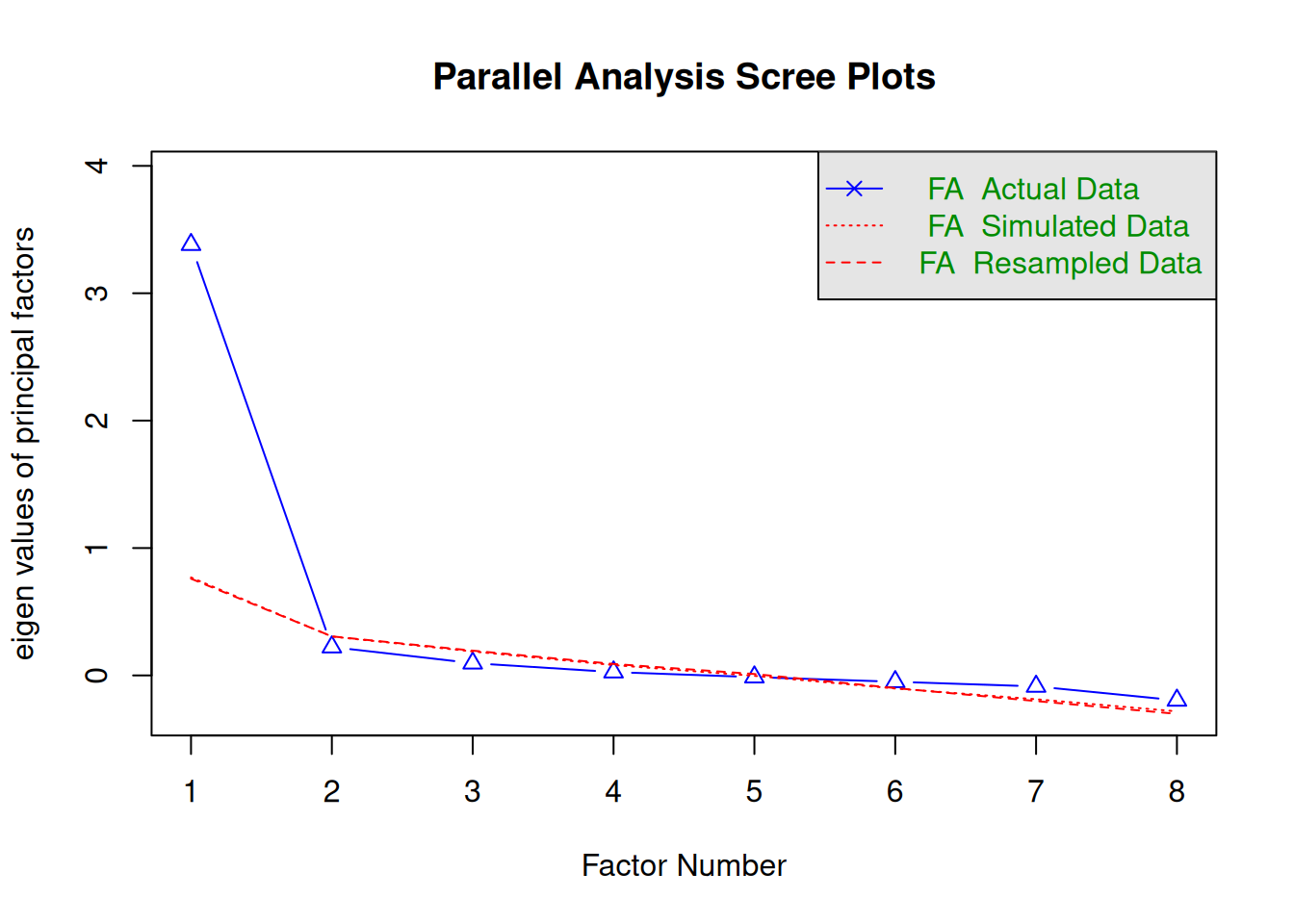
#| fig-cap: "Figure 6.1: Parallel analysis for the candidate short scale."
#| alt: "Parallel analysis for the candidate short scale."
# EFA requires n ≥ 100 ideally; with n=60, results are exploratory only
# Simulate larger dataset for demonstration
efa_data <- chapter6_simulate_scale(
n = 100,
loadings = c(0.82, 0.79, 0.77, 0.74, 0.81, 0.78, 0.76, 0.80),
noise_sd = 0.90,
seed = 2025
)
# Parallel analysis is the key screening plot here; suppress console text in the rendered view
invisible(capture.output(
fa.parallel(efa_data, fa = "fa")
))
# Fit 1-factor model
efa_result <- fa(efa_data, nfactors = 1, rotate = "oblimin", fm = "minres")
```
#### Cell Code
```{webr-r}
#| context: interactive
# EFA requires n ≥ 100 ideally; with n=60, results are exploratory only
# Simulate larger dataset for demonstration
efa_data <- chapter6_simulate_scale(
n = 100,
loadings = c(0.82, 0.79, 0.77, 0.74, 0.81, 0.78, 0.76, 0.80),
noise_sd = 0.90,
seed = 2027
)
# Parallel analysis is the key screening plot here; suppress console text in the rendered view
invisible(capture.output(
fa.parallel(efa_data, fa = "fa")
))
# Fit 1-factor model
efa_result <- fa(efa_data, nfactors = 1, rotate = "oblimin", fm = "minres")
```
:::::
::::
:::: {.content-visible unless-format="html"}
```{r}
#| label: part-c-scale-dev-4
#| fig-align: center
#| fig-cap: "Figure 6.1: Parallel analysis for the candidate short scale."
#| alt: "Parallel analysis for the candidate short scale."
# EFA requires n ≥ 100 ideally; with n=60, results are exploratory only
# Simulate larger dataset for demonstration
efa_data <- chapter6_simulate_scale(
n = 100,
loadings = c(0.82, 0.79, 0.77, 0.74, 0.81, 0.78, 0.76, 0.80),
noise_sd = 0.90,
seed = 2027
)
# Parallel analysis is the key screening plot here; suppress console text in the rendered view
invisible(capture.output(
fa.parallel(efa_data, fa = "fa")
))
# Fit 1-factor model
efa_result <- fa(efa_data, nfactors = 1, rotate = "oblimin", fm = "minres")
```
::::
Figure 6.1 shows the parallel-analysis result for the simulated 8-item scale. In this example, the factor solution is the relevant guide: one factor is retained, and the fitted one-factor model explains about 43.9% of the total variance. Some software also prints a separate "components" recommendation. For early scale development, the factor recommendation is the substantively relevant result [@costello2005].
**Caution**: Even when parallel analysis suggests one dominant factor in a simulated example like this, `n = 100` still only supports **preliminary guidance**. Treat EFA results as provisional until a larger validation sample can confirm the structure. For early psychological scale development, a first factor explaining roughly 40% to 60% of the variance is often acceptable as an initial signal rather than a final validation result [@costello2005].
#### Stage 4: Validation (n = 150+)
**Goal**: Confirm scale structure and establish validity.
In this chapter, `SEM` refers to **structural equation modelling**. In Chapter 5, `SEM` denoted the **standard error of measurement**. The context distinguishes the two uses.
**Methods**:
- **Confirmatory Factor Analysis (CFA)**: Test hypothesized factor structure
- **Test-retest reliability**: Administer scale twice (2–4 weeks apart)
- **Convergent validity**: Correlate with theoretically related measures
- **Discriminant validity**: Show low correlation with unrelated constructs
- **Known-groups validity**: Scale discriminates between relevant groups
**Example**:
```{r}
#| label: part-c-scale-dev-5
#| eval: false
# CFA requires lavaan package and n ≥ 150
library(lavaan)

# Define 1-factor model
model <- '
  resilience =~ WRS1 + WRS2 + WRS3 + WRS4 + WRS5 + WRS6 + WRS7 + WRS8
'

# Fit model
cfa_result <- cfa(model, data = validation_data)
summary(cfa_result, fit.measures = TRUE, standardized = TRUE)

# Fit indices to assess model adequacy (conventional heuristics):
# - CFI >= 0.90 (acceptable), >= 0.95 (good)
# - RMSEA <= 0.08 (acceptable), <= 0.06 (good)
# - SRMR <= 0.08 (acceptable)
# Evaluate fit holistically rather than treating cutoffs as automatic rules.
```
Use these fit indices as heuristics rather than absolute pass-fail rules. CFI compares the hypothesised model with a baseline model in which the items are treated as unrelated. Larger values indicate better relative fit. RMSEA estimates lack of fit per model degree of freedom. Smaller values indicate closer approximate fit. SRMR summarises the average standardised residual discrepancy between the observed and model-implied correlations. Conventional thresholds such as CFI >= 0.95, RMSEA <= 0.06, and SRMR <= 0.08 are useful vocabulary, but they were developed mostly for larger samples and should not be applied mechanically in small validation studies [@hu1999]. If fit is poor, report the indices, inspect the pattern of residuals and loadings, and explain the limitation. Do not repeatedly refit the model until the cutoffs are met.
Some short scales also contain both a broad general construct and narrower item clusters. In that setting, a bifactor model can separate the general factor from group factors and can support omega-hierarchical as an estimate of reliability for the general factor. This is a larger-sample validation tool, not a pilot-stage shortcut.
**Test-retest reliability**:
```{r}
#| label: part-c-scale-dev-6
#| eval: false
# Compute scale scores at Time 1 and Time 2
validation_data <- validation_data %>%
  dplyr::mutate(
    resilience_t1 = rowMeans(dplyr::select(., WRS1_t1:WRS8_t1), na.rm = TRUE),
    resilience_t2 = rowMeans(dplyr::select(., WRS1_t2:WRS8_t2), na.rm = TRUE)
  )

# Intraclass correlation coefficient (ICC)
# Specify the model explicitly because ICC values depend on the chosen form.
library(irr)
icc_result <- icc(
  cbind(validation_data$resilience_t1, validation_data$resilience_t2),
  model = "twoway",
  type = "agreement",
  unit = "single"
)
print(icc_result)

# ICC > 0.75 is often treated as good test-retest reliability,
# but always report the ICC model and confidence interval.
```
When reporting ICC, specify the model and interpretation rule directly in the text. A two-way agreement ICC above about 0.75 is often treated as good evidence of test-retest reliability, but the exact value depends on the ICC form chosen [@cicchetti1994; @koo2016].
### Special Considerations for n < 50
#### What You CANNOT Do
::: {.callout-warning icon=true}
## Analyses That Require Larger Samples
With n < 50, the following analyses are **not feasible** or will produce unreliable results:
1. **Exploratory Factor Analysis (EFA)**: Rule of thumb is n ≥ 100 or 5–10 participants per item
2. **Confirmatory Factor Analysis (CFA)**: Requires n ≥ 150–200 for stable parameter estimates
3. **Measurement Invariance Testing**: Requires n ≥ 200 per group
4. **Structural Equation Modelling (SEM)**: Complex models need n ≥ 200–400
5. **PLS-SEM (Partial Least Squares SEM)**: Despite "small-sample" marketing claims, stable path estimates still usually need at least n ≈ 100–150
6. **Item Response Theory (IRT)**: Most models require n ≥ 250–500
7. **Reliable Cronbach's alpha**: With n < 30, alpha estimates have 95% CIs spanning 0.3–0.4 units
Keep these methods for larger studies. Forced application to very small samples produces misleading results.
:::
---
::: {.callout-note icon=false collapse=true}
## Why Structural Equation Modelling (SEM) Requires Large Samples
**Question**: "Can I use SEM, CFA, or PLS-SEM with my small sample (n < 100)?"
**Short Answer**: **No.** SEM-based methods require substantially larger samples than this book's target range (n = 10–100).
### Minimum Sample Size Requirements
| Method | Minimum n | Realistic n | Why? |
|--------|-----------|-------------|------|
| **Confirmatory Factor Analysis (CFA)** | 150 | 200-300 | Stable factor loadings, fit indices |
| **Structural Equation Modelling (SEM)** | 200 | 300-500 | Complex path models, multiple latent variables |
| **PLS-SEM** | 100 | 150-300 | Despite "small-sample" marketing claims, stable path estimates usually need at least 100-150 cases |
| **Multi-Group SEM** | 200/group | 300/group | Measurement invariance testing |
**Rule of Thumb**: 10-20 observations per estimated parameter is a common starting heuristic (e.g., 5 indicators + 3 paths = 8 parameters → need 80-160 observations), but actual requirements vary with model complexity, indicator quality, and estimation method.
That is why the table above should be read as planning guidance rather than a universal rulebook. Even methods sometimes marketed as "small-sample friendly," such as PLS-SEM, still need enough observations for stable path estimates and standard errors [@hair2017].
### What Happens If You Ignore These Requirements?
With n < 100, SEM/CFA/PLS-SEM tends to produce unstable parameter estimates. Factor loadings can fluctuate sharply after very small data changes, path coefficients often carry very large standard errors, and conclusions may change when only a handful of observations are added or removed.
Small samples also increase the risk of non-convergent or improper solutions. Maximum-likelihood estimation may fail to converge, Heywood cases such as negative variances or loadings above 1.0 become more likely, and analysts can end up imposing arbitrary constraints simply to force the model to run.
Even when the software returns output, the fit statistics are difficult to trust. With small n, χ², CFI, TLI, and RMSEA can look reassuring for the wrong reasons, modification indices often suggest spurious changes, and a model may appear to fit the sample well only because it has overfit noise that will not replicate in new data.
The final danger is false confidence. SEM software will still print parameter estimates, p-values, confidence intervals, and polished path diagrams, but that appearance of technical completeness does not make the results trustworthy. Reviewers and readers will rightly question claims built on latent-variable models that the sample size cannot support.
### What Should You Do Instead? (For n < 100)
**Use the methods in THIS book:**
| SEM Goal | Small-Sample Alternative | Chapter | Minimum n |
|----------|-------------------------|---------|-----------|
| **Assess scale reliability** | Cronbach's α, McDonald's ω, split-half | Ch 6 | 30-50 |
| **Validate items** | Item-total correlations, alpha-if-deleted | Ch 6 | 30-50 |
| **Reduce dimensionality** | **Sum/mean composite scores** | Ch 6 | 20+ |
| **Test relationships (X → Y)** | Regression with composite scores | Ch 5 | 30-50 |
| **Multiple predictors** | Penalized regression (ridge/lasso/elastic net) | Ch 13 | 50-100 |
| **Mediation (X → M → Y)** | Simple mediation with bootstrap CIs | Part E Project 5 | 80-100 |
| **Latent correlations** | Polychoric correlations (exploratory) | Ch 6 | 50+ |
| **Measurement precision** | Standard Error of Measurement (SEM statistic) | Ch 6 | 30+ |
**Key Principle**: **Composite scores are your friend.**
- Sum or average your scale items to create observed composite variables
- Use these composites in regression, t-tests, ANOVA
- Acknowledge measurement error in limitations section
- Plan larger validation study (n ≥ 200) for future CFA/SEM
### Example: Replacing SEM with Composite-Score Analysis
**Proposed SEM Model (n = 60):**
```
Job_Satisfaction (5 items) → Turnover_Intent (3 items)
     ↑
Performance (4 items)
```
**Small-Sample Alternative:**
```{webr-r}
#| context: interactive
# Create a small example dataset with 5 satisfaction, 4 performance,
# and 3 turnover-intention items.
set.seed(2025)
data <- tibble::as_tibble(
matrix(
sample(c(1:5, NA), size = 60 * 12, replace = TRUE, prob = c(rep(0.19, 5), 0.05)),
nrow = 60
)
)
names(data) <- c(
paste0("satisfaction_", 1:5),
paste0("performance_", 1:4),
paste0("turnover_", 1:3)
)
# Create composite scores by averaging items when enough responses are present
data <- data %>%
dplyr::mutate(
satisfaction_missing = rowSums(is.na(dplyr::select(., satisfaction_1:satisfaction_5))),
performance_missing = rowSums(is.na(dplyr::select(., performance_1:performance_4))),
turnover_missing = rowSums(is.na(dplyr::select(., turnover_1:turnover_3))),
satisfaction = ifelse(
satisfaction_missing <= 1,
rowMeans(dplyr::select(., satisfaction_1:satisfaction_5), na.rm = TRUE),
NA_real_
),
performance = ifelse(
performance_missing <= 1,
rowMeans(dplyr::select(., performance_1:performance_4), na.rm = TRUE),
NA_real_
),
turnover = ifelse(
turnover_missing == 0,
rowMeans(dplyr::select(., turnover_1:turnover_3), na.rm = TRUE),
NA_real_
)
)
# Test relationships with standard regression
model1 <- lm(turnover ~ satisfaction, data = data)
model2 <- lm(turnover ~ satisfaction + performance, data = data)
# Report coefficients, R², confidence intervals
```
**Advantages**: This composite-score approach works with n = 60, remains interpretable because coefficients refer to changes in averaged scale scores, and is usually more robust than forcing a latent-variable model onto limited data. It is also more honest, because it acknowledges that observed composites are being analysed directly rather than pretending the sample is large enough for stable latent-variable estimation.
**Limitations to Acknowledge**: Composite scores still contain measurement error, they cannot test complex factor structures, and they do not separate within-item from between-item variance. Missing-data rules also need to be stated explicitly so readers know when partial composites were allowed and when cases were excluded.
**When to Pursue SEM**: Collect n ≥ 200 in a follow-up study. Then:
1. Use EFA to explore factor structure (if theory is unclear)
2. Use CFA to confirm measurement model
3. Test structural paths with latent variables
4. Assess model fit rigorously
### Software Will Let You Do Bad Things
**Warning**: SmartPLS, AMOS, Mplus, and other SEM software will happily run with n = 50. They will produce:
- Parameter estimates
- p-values
- Fit indices
- Pretty path diagrams
**This does NOT mean the results are trustworthy.** Software cannot judge whether your sample size is adequate—**you must.**
### Recommended Reading (For Future Large-Sample Studies)
When you collect n ≥ 200, consult these resources:
1. **Kline, R. B. (2016).** *Principles and Practice of Structural Equation Modeling* (4th ed.). Guilford Press.
- Gold standard SEM textbook
- Sample size guidelines (pp. 15-18, 264-270)
2. **Brown, T. A. (2015).** *Confirmatory Factor Analysis for Applied Research* (2nd ed.). Guilford Press.
- CFA-specific guidance
- Measurement invariance testing
3. **Hair, J. F., Hult, G. T. M., Ringle, C. M., & Sarstedt, M. (2022).** *A Primer on Partial Least Squares Structural Equation Modeling (PLS-SEM)* (3rd ed.). Sage.
- PLS-SEM methods (but note: still needs n ≥ 100-150 realistically)
4. **Hoyle, R. H. (Ed.). (2023).** *Handbook of Structural Equation Modeling* (2nd ed.). Guilford Press.
- Advanced topics, sample size planning
### Bottom Line
For n = 10–100, the methods in this book are the defensible default because they are appropriate for small samples, robust to common assumption problems, honest about uncertainty, and interpretable for substantive readers and reviewers. Save SEM for a later study with n >= 200. Until then, composite scores combined with transparent regression-style analyses will usually serve the research question much better.
:::
---
#### What You CAN Do
With n = 20–50, focus on these **feasible and informative** analyses:
1. **Content validity.** Use expert review, cognitive interviews, and explicit links to the theoretical framework to decide whether the item pool is clear, relevant, and broad enough before you rely on any statistics.
2. **Item-level diagnostics.** Examine item means, standard deviations, skewness, corrected item-total correlations, floor or ceiling effects, and the inter-item correlation matrix to flag items that are obviously misbehaving.
3. **Preliminary reliability (n ≥ 30).** Report Cronbach's alpha with its 95% confidence interval, add split-half reliability as a robustness check, and inspect the mean inter-item correlation to see whether the scale is too loose or too redundant.
4. **Known-groups validity.** Compare scale scores between groups that theory predicts should differ, and use nonparametric methods such as the Mann–Whitney U test if the scale scores are skewed or ordinal.
5. **Preparation for a larger validation study.** Document the item-generation process, report pilot decisions transparently including which items were dropped and why, and use the pilot to specify the hypotheses that a later CFA or validation study will test.
### Example: Documenting a Small-Sample Scale Development
:::: {.content-visible when-format="html"}
::::: {.panel-tabset group="part-c-analysis-methods-chapter-6-5-developing-short-scales-for-small-samples-cell-5"}
#### Rendered Output
```{r}
#| label: part-c-scale-dev-7-html
#| echo: false
#| results: asis
# Reporting template for n < 50 pilot study
scale_dev_report <- tibble(
Stage = c("Item Generation", "Pilot Testing", "Refinement", "Validation"),
Sample_Size = c("n = 8 (cognitive interviews)", "n = 25", "n = 60", "Planned: n = 200"),
Analyses_Conducted = c(
"Think-aloud protocols; expert review (CVI = 0.88)",
"Item-total correlations; ceiling/floor checks; 3 items dropped",
"Alpha = 0.84 [95% CI: 0.77, 0.90]; split-half = 0.79-0.90",
"CFA, test-retest ICC, convergent validity (planned)"
),
Key_Findings = c(
"Generated 15 items; 2 flagged as ambiguous",
"Dropped WRS5 (ceiling), WRS8 (r.cor = 0.10), WRS11 (low variance)",
"8-item scale shows acceptable reliability for research use",
"Pending larger validation sample"
)
)
chapter6_scale_table(
number = "6.4",
title = "Illustrative staged reporting summary for a short-scale development project.",
data = scale_dev_report %>%
dplyr::rename(
`Development Stage` = Stage,
`Sample Size` = Sample_Size,
`Analyses Conducted` = Analyses_Conducted,
`Key Findings` = Key_Findings
),
note = "Report the actual pilot sample sizes, item deletions, and planned validation targets transparently.",
align = c("l", "l", "l", "l")
)
```
#### Cell Code
```{webr-r}
#| context: interactive
# Reporting template for n < 50 pilot study
scale_dev_report <- tibble(
Stage = c("Item Generation", "Pilot Testing", "Refinement", "Validation"),
Sample_Size = c("n = 8 (cognitive interviews)", "n = 25", "n = 60", "Planned: n = 200"),
Analyses_Conducted = c(
"Think-aloud protocols; expert review (CVI = 0.88)",
"Item-total correlations; ceiling/floor checks; 3 items dropped",
"Alpha = 0.84 [95% CI: 0.77, 0.90]; split-half = 0.79-0.90",
"CFA, test-retest ICC, convergent validity (planned)"
),
Key_Findings = c(
"Generated 15 items; 2 flagged as ambiguous",
"Dropped WRS5 (ceiling), WRS8 (r.cor = 0.10), WRS11 (low variance)",
"8-item scale shows acceptable reliability for research use",
"Pending larger validation sample"
)
)
chapter6_scale_table(
number = "6.4",
title = "Illustrative staged reporting summary for a short-scale development project.",
data = scale_dev_report %>%
dplyr::rename(
`Development Stage` = Stage,
`Sample Size` = Sample_Size,
`Analyses Conducted` = Analyses_Conducted,
`Key Findings` = Key_Findings
),
note = "Report the actual pilot sample sizes, item deletions, and planned validation targets transparently.",
align = c("l", "l", "l", "l")
)
```
:::::
::::
:::: {.content-visible unless-format="html"}
```{r}
#| label: part-c-scale-dev-7
#| results: asis
# Reporting template for n < 50 pilot study
scale_dev_report <- tibble(
Stage = c("Item Generation", "Pilot Testing", "Refinement", "Validation"),
Sample_Size = c("n = 8 (cognitive interviews)", "n = 25", "n = 60", "Planned: n = 200"),
Analyses_Conducted = c(
"Think-aloud protocols; expert review (CVI = 0.88)",
"Item-total correlations; ceiling/floor checks; 3 items dropped",
"Alpha = 0.84 [95% CI: 0.77, 0.90]; split-half = 0.79-0.90",
"CFA, test-retest ICC, convergent validity (planned)"
),
Key_Findings = c(
"Generated 15 items; 2 flagged as ambiguous",
"Dropped WRS5 (ceiling), WRS8 (r.cor = 0.10), WRS11 (low variance)",
"8-item scale shows acceptable reliability for research use",
"Pending larger validation sample"
)
)
chapter6_scale_table(
number = "6.4",
title = "Illustrative staged reporting summary for a short-scale development project.",
data = scale_dev_report %>%
dplyr::rename(
`Development Stage` = Stage,
`Sample Size` = Sample_Size,
`Analyses Conducted` = Analyses_Conducted,
`Key Findings` = Key_Findings
),
note = "Report the actual pilot sample sizes, item deletions, and planned validation targets transparently.",
align = c("l", "l", "l", "l")
)
```
::::
### Reporting Guidelines for Small-Sample Scale Development
When publishing or reporting scale development work with n < 50:
1. **Acknowledge limitations explicitly**:
- "With n = 25, we could not reliably estimate Cronbach's alpha. Instead, we focused on item-total correlations to identify weak items."
- "Exploratory factor analysis was not feasible (n = 60); we plan CFA with a larger sample (target n = 200)."
2. **Report what you did (not what you wish you could do)**:
Avoid presenting alpha as a definitive reliability estimate when n < 30. If a journal requires it, report the confidence interval and describe the result as preliminary screening information. Do not force EFA or CFA with inadequate samples. Instead, explain the theoretical rationale for the proposed item grouping and reserve the structural test for a later study.
3. **Frame as a preliminary/pilot study**:
State plainly that the work is a pilot or refinement study and explain what that means for interpretation. For example: "This pilot study (n = 35) was designed to refine item wording and identify problematic items before a larger validation study," or "Results are preliminary and should be interpreted with caution pending validation with n ≥ 150."
4. **Provide detailed item-level information**:
- Publish item means, SDs, item-total correlations
- Report which items were dropped and why
- Share cognitive interview feedback (qualitative)
5. **Plan and fund the validation study**:
- Use pilot data to justify sample size for validation (power analysis for CFA)
- Secure resources for n ≥ 150–200 before claiming a "validated" scale
### Key Takeaways
Scale development with small samples is best understood as a staged process rather than a single psychometric event. Very small pilots are most useful for qualitative refinement and item-level diagnostics, somewhat larger samples can support cautious preliminary reliability work, and only much larger studies can justify structural validation through EFA, CFA, and broader validity testing. Across all of those stages, transparency about what was and was not feasible is what makes the evidence credible.
---
### Self-Assessment Quiz
```{r}
#| echo: false
#| results: asis
source(normalizePath(file.path(dirname(knitr::current_input(dir = TRUE)), "..", "R", "quiz_helpers.R"), mustWork = TRUE))
smallsamplelab_render_quiz(list(
list(
prompt = "Why is scale development with small samples best treated as a multi-stage process?",
options = c("Because all psychometric evidence can be collected from one pilot sample", "Because different stages support different goals, from item clarity to later validation, and each requires different sample sizes", "Because short scales never need validation", "Because only qualitative methods are allowed with small samples"),
answer = 2L,
explanation = "The chapter presents scale development as an iterative process. Early stages focus on item generation and pilot diagnostics, while later stages support reliability estimation, factor analysis, and validation. Small samples can support some of these steps, but not all of them at once."
),
list(
prompt = "At the item-generation stage, what is the main priority?",
options = c("Estimating Cronbach's alpha", "Running confirmatory factor analysis", "Checking whether items are clear, relevant, and comprehensible through literature review, expert consultation, and cognitive interviews", "Computing test-retest reliability"),
answer = 3L,
explanation = "Stage 1 emphasises item generation and comprehension. The chapter explicitly states that this stage should focus on literature review, expert consultation, and cognitive interviews rather than quantitative psychometric estimation."
),
list(
prompt = "With a pilot sample of about 20 to 30 participants, which analysis is most appropriate?",
options = c("A full CFA with fit indices", "Item-total correlations, ceiling or floor checks, and item means and SDs", "A definitive test-retest reliability study", "A published claim that the scale is fully validated"),
answer = 2L,
explanation = "The chapter recommends item-level diagnostics at the pilot stage: item-total correlations, ceiling and floor checks, and basic descriptive statistics. These analyses help identify weak items before larger validation work."
),
list(
prompt = "Why does the chapter warn against relying on Cronbach's alpha with n < 30?",
options = c("Alpha cannot be computed in R", "Alpha estimates are highly unstable and have very wide confidence intervals with such small samples", "Alpha is only for binary items", "Alpha is irrelevant for short scales"),
answer = 2L,
explanation = "The warning callout explains that alpha estimates are highly unstable with n < 30, making the confidence interval so wide that the estimate is not very informative for decision-making."
),
list(
prompt = "What should you do when an item shows a ceiling effect in the pilot data?",
options = c("Automatically keep it because everyone agrees", "Remove or reword it because respondents are not differentiating on that item", "Use CFA immediately", "Average it with another item"),
answer = 2L,
explanation = "The chapter's pilot example flags ceiling effects as a sign that an item may not discriminate well. The recommended response is to remove or reword the item."
),
list(
prompt = "At roughly what stage does the chapter consider exploratory factor analysis potentially feasible?",
options = c("Immediately after cognitive interviews", "At the refinement stage, ideally when n approaches or exceeds 100, and even then results are tentative with modest samples", "Only after test-retest reliability", "Never in small-sample research"),
answer = 2L,
explanation = "The chapter states that EFA is more defensible at the refinement stage and ideally with n around 100 or more. With smaller samples, the results are described as exploratory and unstable."
),
list(
prompt = "What is the main goal of the validation stage?",
options = c("To decide whether items are comprehensible", "To confirm scale structure and establish validity evidence such as CFA, test-retest reliability, and convergent validity", "To compute item means only", "To avoid collecting any more data"),
answer = 2L,
explanation = "Stage 4 is the validation phase. It is where the chapter places confirmatory factor analysis, test-retest reliability, convergent validity, discriminant validity, and known-groups validity."
),
list(
prompt = "Which reporting practice best fits a pilot scale-development study with n = 35?",
options = c("Claim the scale is fully validated", "Report preliminary item-level diagnostics, acknowledge the limitations, and state that larger-sample validation is still needed", "Suppress the sample size because it looks weak", "Present CFA fit indices from an underpowered model as definitive evidence"),
answer = 2L,
explanation = "The reporting guidelines emphasise honesty about what the study could and could not show. With a pilot sample, the chapter recommends framing findings as preliminary and stating the need for a larger validation study."
),
list(
prompt = "Why is transparency especially important in small-sample scale development?",
options = c("Because reviewers ignore sample sizes", "Because readers need to know which psychometric claims are supported now and which must wait for later validation", "Because short scales do not need theory", "Because only qualitative evidence matters"),
answer = 2L,
explanation = "The chapter repeatedly stresses transparency: report what you did, what you did not do, and why. Small samples can support useful refinement decisions, but they do not justify overclaiming full validation."
),
list(
prompt = "Which conclusion is most consistent with the chapter's overall message?",
options = c("A small pilot sample can fully validate a new instrument", "Scale development with small samples can be rigorous if it proceeds in stages and reserves stronger psychometric claims for later, larger studies", "Factor analysis is always mandatory before any scale can be used", "Item wording matters less than alpha"),
answer = 2L,
explanation = "Small samples require staged, realistic claims. Early work can be rigorous when researchers match their analyses to the evidence their sample can support, even if full validation must wait for a larger dataset."
)
))
```