Chapter 2: Questions and Outcomes that Fit Small n
Small-sample studies are most effective when the research question, outcome, and design are chosen to match the information the data can realistically support. This chapter shows how to narrow broad ideas into answerable questions, how outcome scales affect what can be learned from modest samples, and why estimation often matters more than a binary significant or non-significant result. The goal is practical: to help you design studies that extract the most from limited data and communicate findings at a level the evidence can honestly support.
Learning Objectives
By the end of this chapter, you will be able to distinguish exploratory from confirmatory aims, formulate focused research questions that fit limited data, choose outcome measures that preserve useful information with small n, and calculate the minimum detectable effects implied by a realistic design.
Framing Realistic Research Questions
Small-sample studies work best when the research question is narrow. Questions that ask the data to estimate many predictors, interactions, mediation paths, or measurement parameters such as factor loadings for a long questionnaire usually require far more observations. Focused questions about a single outcome or a few key comparisons are much more realistic with modest samples.
When planning a small-sample study, prioritise clarity and specificity. A question such as “Does a brief reminder intervention improve adherence compared to standard care?” is focused, has a clear comparison, and can be tested in a small randomised trial. A question like “What are all the factors that influence patient adherence?” spreads the available information across too many unknowns.
Similarly, consider whether the study is exploratory or confirmatory. Exploratory studies generate hypotheses, describe patterns, and refine measurement instruments. They can be useful with modest samples, provided the findings are framed as provisional and replication is expected. Because exploratory work often examines several patterns at once, apparent findings may reflect chance, especially when researchers inspect several outcomes or subgroup patterns without adjustment. Confirmatory studies test prespecified hypotheses and therefore require enough power to support that stronger claim. With small samples, confirmatory aims should be modest and carefully justified.
From Objective to Hypothesis
A small-sample study benefits from a clear hierarchy. In a confirmatory design, that usually means one primary objective, one primary research question, and one primary hypothesis. In an exploratory or pilot design, the hypothesis is often replaced with an estimation or feasibility objective because the data cannot support several formal confirmatory claims well. The objective states what the study is trying to learn, the research question identifies the population, comparison, outcome, and timeframe, and the hypothesis states the expected difference or association on that specific outcome.
For example, a focused small-sample study might use the following sequence:
- Objective: To assess whether a brief reminder intervention improves medication adherence over four weeks compared with standard care.
- Research question: Among adults attending a primary-care clinic, do participants receiving the reminder intervention have higher four-week adherence scores than those receiving standard care?
- Confirmatory hypothesis: Participants assigned to the reminder intervention will have higher mean adherence scores at four weeks than participants assigned to standard care.
- Exploratory objective: To estimate the difference in adherence score between groups and assess recruitment, retention, and intervention uptake in preparation for a larger confirmatory trial.
When writing hypotheses for small-sample studies, keep them narrow and defensible. A good small-sample hypothesis names one primary outcome, one main comparison, and a plausible expected pattern. Directional hypotheses are best reserved for situations where prior theory or evidence is strong enough to justify specifying the direction in advance. Avoid omnibus statements that bundle several outcomes, subgroup effects, mediators, and interactions into a single claim. Avoid phrasing hypotheses around achieving statistical significance. The hypothesis should describe the expected substantive pattern, while the analysis later evaluates its uncertainty.
Choosing Appropriate Outcomes
The type of outcome variable influences which methods are feasible and how much information can be extracted from limited data. Binary outcomes (yes/no, success/failure) are common but carry less information per observation than continuous or ordinal measures. If your sample is small, consider whether a continuous or ordinal outcome might capture more variation and yield more precise inferences.
For example, rather than dichotomising patient improvement into “improved” versus “not improved”, use a continuous measure of symptom severity or an ordinal scale with several levels. This preserves information and increases statistical efficiency. When the outcome is inherently binary, such as survival within 30 days, keep it in that form.
Count outcomes (number of adverse events, number of customer complaints) are also informative but may be sparse when samples are small. Exact Poisson tests and negative binomial models can handle low counts, but very sparse data (many zeros, few events) may require careful interpretation or resampling methods.
Outcome Selection Decision Guide
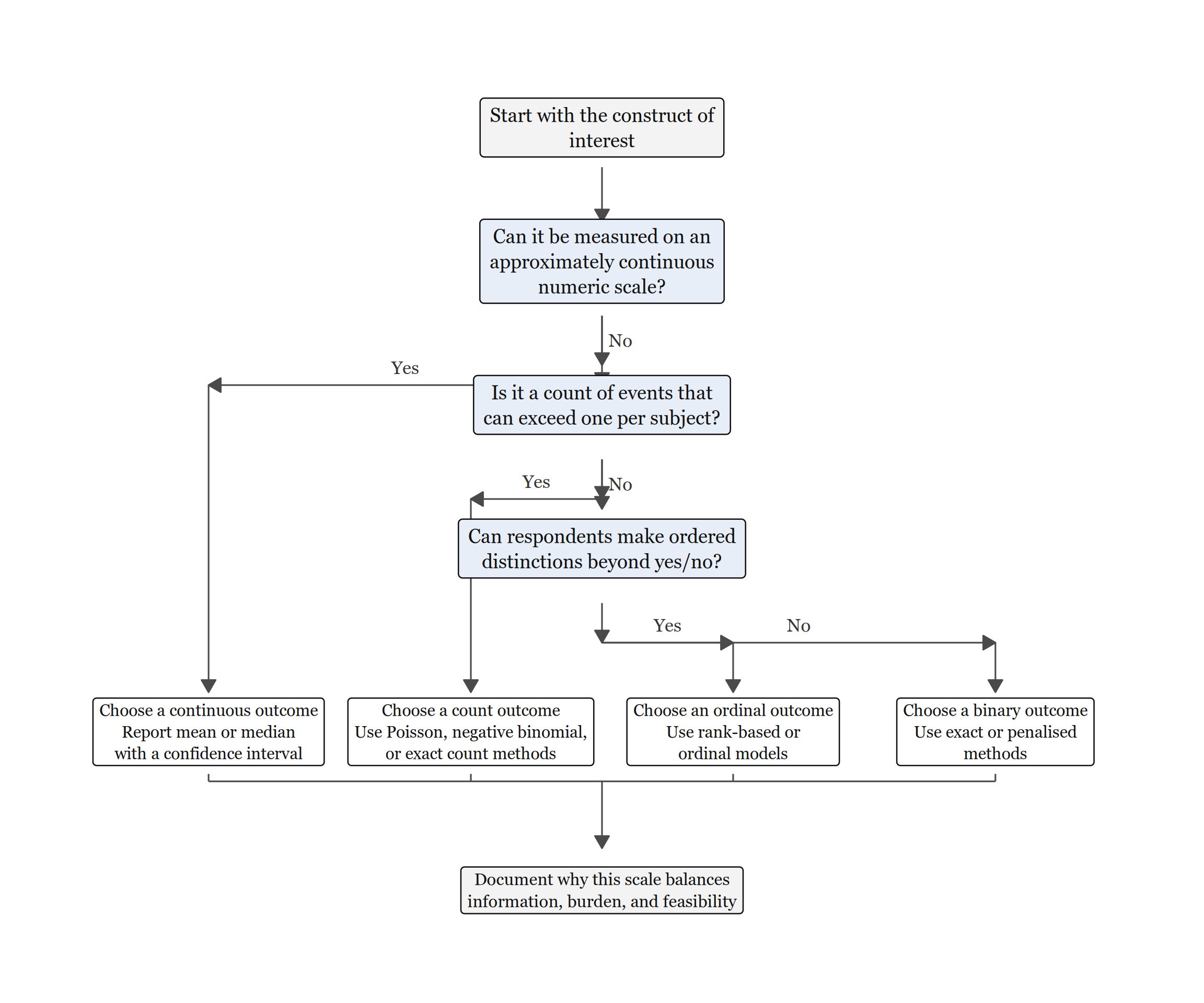
Figure 2.1 turns outcome selection into a sequence of questions. It starts with the construct itself, then separates continuous, count, ordinal, and binary outcomes in the order that preserves the most defensible information from small samples.
Read Figure 2.1 from top to bottom. The ambiguous cases usually arise between ordinal and binary coding, or between count outcomes and simpler event/no-event summaries. The guiding principle is to keep the scale that preserves the most defensible information. Binary coding is still appropriate when the construct genuinely has only two meaningful states, or when the substantive decision itself is binary. After choosing the outcome family, explain why that scale balances information, measurement burden, and feasibility for the study.
Effect Sizes and Estimation
In small-sample research, point estimates of effect sizes (differences in means, odds ratios, correlation coefficients) are often more useful than p-values alone. Even when a small sample has limited power, the estimated effect size and its confidence interval indicate the likely magnitude and precision of the effect.
A non-significant result in a small study does not by itself imply that the effect is trivial or absent. It may simply indicate that the data are not precise enough to distinguish a moderate effect from zero with confidence.
When reporting results, emphasise effect sizes and uncertainty intervals. For example, “The mean difference in satisfaction scores was 1.5 points (95% CI: 0.5 to 2.5)” is more informative than “The difference was statistically significant (p = 0.03)”. Effect size estimates help readers judge practical importance and facilitate meta-analysis or future sample size planning. When the sample size is fixed in advance, it is also useful to report the minimum detectable effect: the smallest effect your study would be well-positioned to detect under the planned design.
For example, if a two-group study is limited to 15 participants per group and targets 80% power under a two-sided \(\alpha = 0.05\), the minimum detectable standardised effect is approximately d = 1.06. That means the study is only sensitive to very large differences. Under the same two-sided \(\alpha = 0.05\) and 80% power assumptions, detecting a small effect such as d = 0.2 would require about 393 participants per group. Thinking in terms of minimum detectable effects helps researchers decide whether a question is realistically answerable with the sample size they can obtain.
As a practical planning check, suppose your budget allows n = 20 per group and the planned analysis is a two-sample t-test with two-sided \(\alpha = 0.05\) and 80% power. The design is only well positioned to detect about d = 0.91 or larger. The next question is substantive rather than computational: would a difference of nearly one pooled standard deviation be the smallest effect worth detecting in your field? If the answer is no, the honest options are to narrow the question, improve measurement precision, use a more efficient paired or stratified design, or frame the study as exploratory rather than confirmatory.
Example: Outcome Selection in a Pilot Study
Suppose you are evaluating a pilot training programme with 18 participants. You have two outcome options: (1) binary pass/fail on a final assessment, or (2) a continuous score (0–100) on the same assessment.
With the continuous score, the sample mean is 69.9 points and the standard deviation is 8.4, with a 95% confidence interval from 65.7 to 74.0. If we dichotomise the same data, the pass rate is 17 out of 18, or 94.4%, with an exact 95% confidence interval from 72.7% to 99.9%. The binary summary still gives a pass rate and its uncertainty, but it no longer shows how far above or below the threshold participants scored.
Research Design Considerations
Small-sample studies benefit from tight experimental control. Paired or matched designs (before–after, crossover, matched-pair comparisons) reduce variability by comparing each unit to itself or a closely matched control. This within-unit comparison can yield precise inferences even when the number of units is small.
Stratification and blocking can also improve efficiency by accounting for known sources of variation. For example, if you are comparing two teaching methods in a small class, stratify by prior achievement level to reduce heterogeneity within each comparison.
Finally, consider sequential or adaptive designs if feasible. Rather than committing to a fixed sample size in advance, you might prespecify an interim review to decide whether recruitment is working as planned, whether variance estimates are much larger than expected, or whether the study should stop early because the signal is already clear. Bayesian methods are well-suited to this style of design because posterior distributions update naturally as data accumulate: the posterior after the first wave becomes the evidence base that is updated when the next wave arrives. These designs still require advance decision rules and transparent reporting so that flexibility remains planned rather than ad hoc.
Designing Pilot Studies
Pilot studies serve specific purposes: assessing feasibility (recruitment rates, attrition, protocol adherence), refining measurement instruments, and estimating variability to inform future sample size calculations. With very small n (often 10–30 participants), focus on collecting process metrics and precision estimates rather than hypothesis testing. Report:
- Primary feasibility outcomes (e.g., proportion screened who consent, time to complete assessments).
- Preliminary effect estimates with wide confidence intervals, making clear that they are exploratory.
- Adaptations for the main study, especially where procedures proved onerous or data quality issues emerged; describe what was changed and why so that reviewers can see how the pilot informed the main design.
In planning terms, choose a pilot sample large enough to detect major logistical problems (often 12–20 per arm is sufficient for estimating key feasibility parameters rather than testing efficacy), prespecify success criteria such as an acceptable recruitment rate, and plan in advance how you will decide whether to proceed to a full trial (Teare et al. 2014).
Key Takeaways
Small-sample studies work best when the question is narrow, the design is realistic, and the outcome preserves as much defensible information as possible. Exploratory aims, continuous or ordinal measures, and efficient designs such as paired or stratified comparisons often make limited data more informative than an overly ambitious confirmatory plan would. Throughout the design process, report effect sizes and confidence intervals alongside power or feasibility considerations so readers can judge what the study could genuinely show.
Self-Assessment Quiz
Test your understanding of the key concepts from Chapter 2.
Question 1. Which research question is better suited to small samples?
Explanation.
Focused comparative questions with a single primary outcome are feasible with small samples. Multivariate questions (A, C, D) require large samples to estimate many parameters reliably. The chapter emphasizes: “focused questions about a single outcome or a few key comparisons can often be addressed with modest samples.”
Question 2. An exploratory study (n=20) finds that meditation reduces anxiety (p=0.04, d=0.7). How should this be framed?
Explanation.
Exploratory studies with small samples are useful for generating hypotheses, but their findings should be treated as provisional. The chapter emphasizes that such results should be interpreted cautiously, especially because exploratory work can surface patterns that reflect chance and therefore require replication.
Question 3. A researcher dichotomizes a continuous outcome (0–100 scale) into “high” (70 or above) vs “low” (<70). With n=25, what is the consequence?
Explanation.
Dichotomizing continuous variables discards information about the magnitude of differences, reduces statistical power, and can create spurious findings at arbitrary cut-points. The chapter clearly states: “rather than dichotomising patient improvement into ‘improved’ versus ‘not improved’, use a continuous measure… This preserves information and increases statistical efficiency.”
Question 4. A study aims to detect a “small” effect (d=0.2) with 80% power. Approximately how many participants per group are needed?
Explanation.
Detecting small effects requires large samples. For d=0.2 with 80% power and alpha = 0.05 (two-tailed), approximately n=393 per group is needed. With n = 15 per group, the chapter shows that a study is only positioned to detect very large effects, approximately d = 1.06 or larger. This aligns with the power curve in Chapter 1, where the d = 0.3 curve remains well below the conventional power target across typical small-sample settings.
Question 5. Which statement about pilot studies is CORRECT?
Explanation.
Pilot studies (typically n=10-30) assess feasibility (recruitment rates, protocol adherence, measurement properties), refine procedures, and provide preliminary effect size estimates for sample size planning, but are not sufficiently large for definitive hypothesis testing. The chapter’s “Designing Pilot Studies” section explicitly states: “focus on collecting process metrics and precision estimates rather than hypothesis testing.”
Question 6. A researcher plans a study with n=15 per group but calculates they need n=50 per group for 80% power. What should they do?
Explanation.
When the feasible sample size is much smaller than the confirmatory target, the chapter’s guidance is to narrow the claim, treat the work as exploratory or pilot-based, and report what effect sizes the study can realistically detect. That combines the framing guidance from the opening section with the emphasis on minimum detectable effects in the estimation section.
Question 7. Which outcome is LEAST appropriate for n=20?
Explanation.
A 50-item factor analysis asks the data to estimate far too many relationships for n=20. That makes the model unstable and the results difficult to trust. This follows the chapter’s broader point that complex multivariate questions are usually unrealistic with very small samples.
Question 8. A study comparing two teaching methods (n=12 per class) finds no significant difference (p=0.18, d=0.45). The conclusion should be:
Explanation.
With small samples, a non-significant result means the study did not provide clear evidence of a difference. An observed effect of d = 0.45 may still be practically meaningful, and the study lacked power to detect it definitively. The chapter emphasizes: “Even when a small sample has limited power, the estimated effect size and its confidence interval indicate the likely magnitude and precision of the effect.”
Question 9. When choosing between a paired and independent-groups design with small samples, which is generally preferable?
Explanation.
Paired designs reduce within-subject variability and increase power. The chapter’s “Research Design Considerations” section states: “Paired or matched designs (before–after, crossover, matched-pair comparisons) reduce variability by comparing each unit to itself or a closely matched control. This within-unit comparison can yield precise inferences even when the number of units is small.”
Question 10. A pilot study with n=18 yields a mean difference of 5 points (95% CI: [0.2, 9.8]). What is the appropriate next step?
Explanation.
Use this estimate to plan a fully-powered confirmatory study. Pilot studies provide preliminary effect estimates and variability information needed for sample size planning. The chapter recommends reporting preliminary effect estimates with wide confidence intervals, making clear that they are exploratory, and using pilots to estimate variability for future sample size calculations.